Multirate Filtering for Digital Signal Processing: MATLAB® Applications, Chapter 8: Complementary Filter Pairs - Exercises
Contents
Exercise 8.1
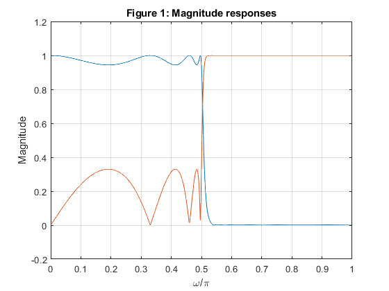
Design the 7th-order elliptic lowpass filter with the passband ripple
ap = 0.5 dB, the stoppband attenuation
as = 50 dB.
Use the function tf2ca to decompose the filter transfer functions into two allpass functions
A0(z) and A1(z).
Combine A0(z) and A1(z) to generate the transfer function
of the complementary highpass filter.
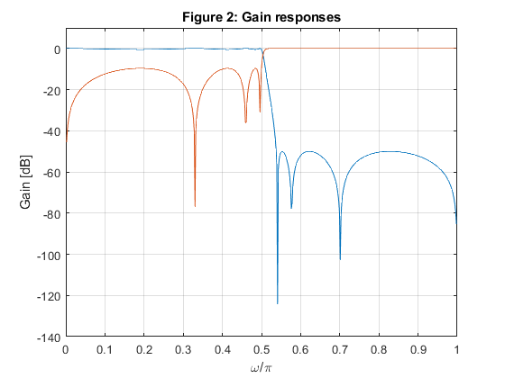
Plot the magnitude responses of the two complementary filters.
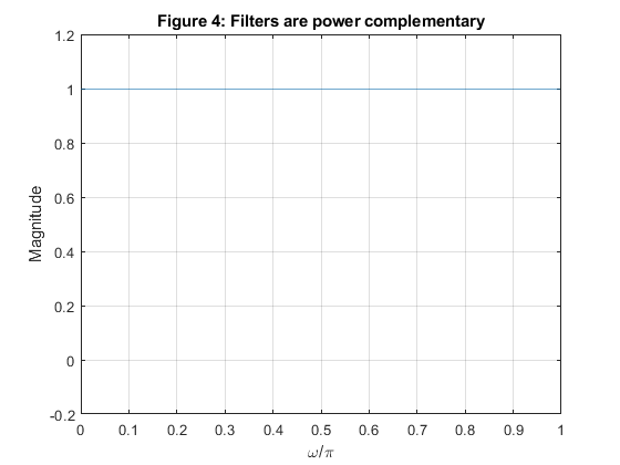
Verify numerically the all-pass complementary and power-complementary
properties.
Used function: ellip, tf2ca, freqz (Signal Processing Toolbox)
clear, close all;
Nord = 7;  ap = 0.5;  as = 50;  fc=0.5;                 % Setting the input parameters
[b,a] = ellip(Nord,ap,as,fc);                           % Design of the LP elliptic filter
[a0dn,a1dn]=tf2ca(b,a);                                 % Calculating coeficients of the allpass filters
[A0,w] = freqz(fliplr(a0dn),a0dn);                      % Frequency response of the A0 allpass filter
[A1,w] = freqz(fliplr(a1dn),a1dn);                      % Frequency response of the A1 allpass filter
% Results
Hlp = (A0+A1)/2;
Hhp = (A0-A1)/2;
figure (1),plot(w/pi,[abs(Hlp) abs(Hhp)]),xlabel('\omega/\pi'),ylabel('Magnitude'),ylim([-0.2 1.2]),grid on
title('Figure 1: Magnitude responses');
figure (2),plot(w/pi,20*log10([abs(Hlp) abs(Hhp)])),xlabel('\omega/\pi'),ylabel('Gain [dB]'),ylim([-140 10]),grid on
title('Figure 2: Gain responses');
figure (3),plot(w/pi,abs(Hlp+Hhp)),xlabel('\omega/\pi'),ylabel('Magnitude'),ylim([-0.2 1.2]),grid on
title('Figure 3: Filters are allpass complementary');
figure (4),plot(w/pi,abs(Hlp).^2+abs(Hhp).^2),xlabel('\omega/\pi'),ylabel('Magnitude'),ylim([-0.2 1.2]),grid on
title('Figure 4: Filters are power complementary');

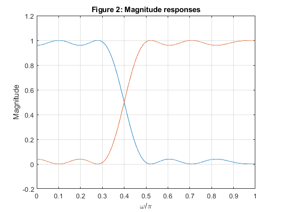
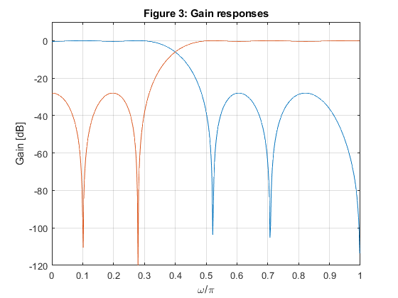
Exercise 8.2
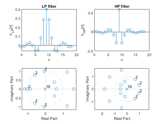
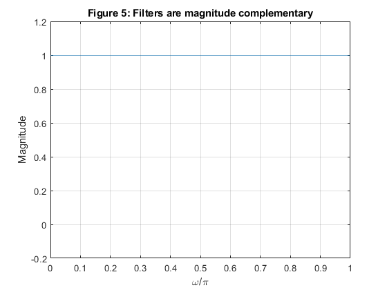
Design a double-complementary (delay-complementary and magnitude complementary)
lowpass/highpass FIR filter pair [HLP(z), HHP(z)] to meet the following specifications:
Filter order Nord = 18, the passband/stopband ripple δ = 0.04,
the crossover frequency ωc = 0.4π.
Plot the following characteristics of
HLP(z), HHP(z):
(i) impulse responses,
(ii) locations of poles and zeros,
(iii) magnitude responses.
Used function: firceqrip (Filter Design Toolbox)
clear, close all;
Nord = 18;  delta = 0.04;  fc = 0.4;                    % Setting the input parameters
delp = delta/(2*(1 - delta));                           % Adjusting the ripple value, Step 1
elp = firceqrip(Nord,fc,[delp,delp]);                   % Design of the intermediate filter Elp(z), Step 2
hlp = (1 - delta)*elp;                                  % Modifying the intermediate filter Elp(z), Step 3
hlp(Nord/2 + 1) = hlp(Nord/2+1)+delta/2;                % Modifying the intermediate filter Elp(z), Step 3
hhp = zeros(size(1:length(hlp)));                       % Zero settings
hhp(10) = 1;  hhp = hhp - hlp;
% Results
figure (1)
subplot(2,2,1),stem([0:Nord],hlp),xlabel('n'),ylabel('h_{LP}[n]'),title('LP filter');
subplot(2,2,2),stem([0:Nord],hhp),xlabel('n'),ylabel('h_{HP}[n]'),title('HP filter');
subplot(2,2,3),zplane(hlp);
subplot(2,2,4),zplane(hhp);
[Hlp,w]=freqz(hlp,1);                                   % Frequency response of the LP filter
[Hhp,w]=freqz(hhp,1);                                   % Frequency response of the HP filter
figure (2)
plot(w/pi,[abs(Hlp) abs(Hhp)]),xlabel('\omega/\pi'),ylabel('Magnitude'),ylim([-0.2 1.2]),grid on,title('Figure 2: Magnitude responses');
figure (3)
plot(w/pi,20*log10([abs(Hlp) abs(Hhp)])),xlabel('\omega/\pi'),ylabel('Gain [dB]'),ylim([-120 10]),grid on,title('Figure 3: Gain responses');
figure (4)
plot(w/pi,abs(Hlp+Hhp)),xlabel('\omega/\pi'),ylabel('Magnitude'),ylim([-0.2 1.2]),grid on,title('Figure 4: Filters are delay complementary');
figure (5)
plot(w/pi,abs(Hlp)+abs(Hhp)),xlabel('\omega/\pi'),ylabel('Magnitude'),ylim([-0.2 1.2]),grid on,title('Figure 5: Filters are magnitude complementary');

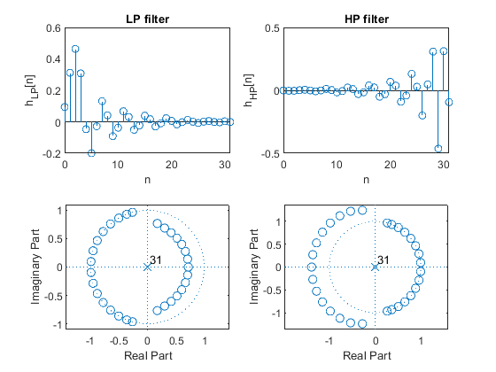
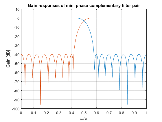
Exercise 8.3
Modify Example 8.2
to design a power-complementary FIR halfband filter pair for the following specifications:
Filter order Nord = 31, the passband/stopband ripple
δ = 0.01, the crossover frequency ωc = 0.5π.
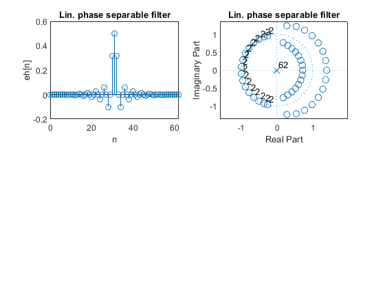
Plot the following characteristics of HLP(z), HHP(z):
(i) impulse responses,
(ii) locations of poles and zeros,
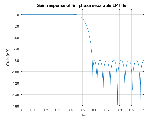
(iii) gain responses.
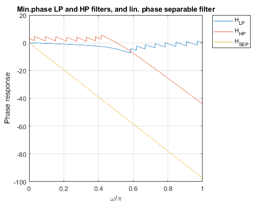
Plot the impulse response, pole-zero locations and the gain response of the
linear-phase separable filter HSEP(z).
Used functions: firceqrip (DSP System Toolbox), minphase (Appendix)
clear, close all;
Nord = 31;  Nord = 2*Nord;  delta = 0.01;               % Setting the input papameters
dfir = (delta^2)/(2*(1 - (delta^2)));                   % Adjusting the ripple value, Substep 1.1
elp = firceqrip(Nord,0.5,[dfir,dfir]);                  % Design of the intermediate filter Elp(z), Substep 1.2
eh = (1-(delta^2))* elp;                                % Modifying the intermediate filter Elp(z), Substep 1.3
eh(Nord/2+1) = eh(Nord/2 + 1) + (delta^2)/2;            % Modifying the intermediate filter Elp(z), Substep 1.3
[hlp,ssp,iter] = minphase(eh(Nord/2 + 1:Nord+1));       % Generating the minimum-phase lowpass filter Hlp(z), Step 2
n = 0:length(hlp) - 1;                                  % Indexing the filter coefficients
hhp = fliplr(hlp).*((-1).^n);                           % Complementary highpass filter, Step 3
% Results
figure (1)
subplot(2,2,1),stem([0:Nord/2],hlp),xlabel('n'),ylabel('h_{LP}[n]');
title('LP filter')
subplot(2,2,2),stem([0:Nord/2],hhp),xlabel('n'),ylabel('h_{HP}[n]');
title('HP filter')
subplot(2,2,3),zplane(hlp);
subplot(2,2,4),zplane(hhp);
[Hlp,w]=freqz(hlp,1);                                   % Frequency response of the LP filter
[Hhp,w]=freqz(hhp,1);                                   % Frequency response of the HP filter
figure (2)
plot(w/pi,20*log10([abs(Hlp) abs(Hhp)])),xlabel('\omega/\pi'),ylabel('Gain [dB]'),grid on;
ylim([-100 10]), title('Gain responses of min. phase complementary filter pair')
[HSEP,w]=freqz(eh,1);                                   % Frequency response of the separable filter
figure (3)
subplot(2,2,1),stem([0:Nord],eh),xlabel('n'),ylabel('eh[n]');
title('Lin. phase separable filter')
subplot(2,2,2),zplane(eh);
title('Lin. phase separable filter')
figure (4)
plot(w/pi,20*log10(abs(HSEP))),xlabel('\omega/\pi'),ylabel('Gain [dB]');
ylim([-160 10]),grid on,title('Gain response of lin. phase separable LP filter')
figure (5)
plot(w/pi,unwrap(angle([Hlp Hhp HSEP]))),xlabel('\omega/\pi'),ylabel('Phase response'),grid on,legend('H_{LP}','H_{HP}','H_{SEP}','Location','NorthEastOutside');
title('Min.phase LP and HP filters, and lin. phase separable filter')
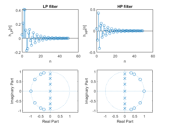
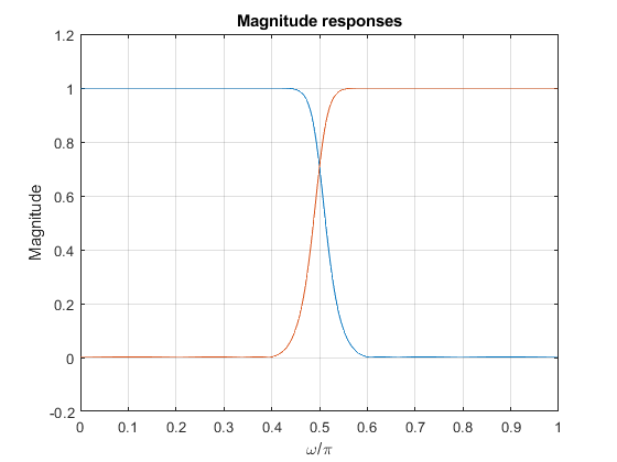
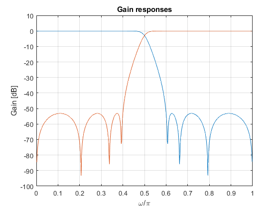
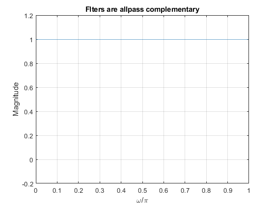
Exercise 8.4
Modify Example 8.3
to design a double-complementary IIR halfnand filter pair for the
following specifications:
Filter order N = 7, the passband edge frequency ωp = 0.5π.
Plot the following characteristics of lowpass and highpass filters HLP(z), HHP(z):
(i) the first 50 samples of impulse responses,
(ii) locations of poles and zeros,
(iii) gain responses.
For the designed filter pair verify power complementary and all-pass complementary properties.
Used function: halfbandiir (Appendix)
clear, close all;
N = 7;  fp = 0.4;                                       % Setting input parameters for lowpass filter
[b,a,z,p,k] = halfbandiir(N,fp);                        % Lowpass halfband filter design
pabs = sort(abs(p));                                    % Order of the filter poles
beta01 = (abs(pabs(2)))^2;
beta11 = (abs(pabs(4)))^2;
beta02 = (abs(pabs(6)))^2;                              % Coefficients of allpass branches
a0nom = conv([beta01 0 1],[beta02 0 1]);
a0denom = conv([1 0 beta01],[1 0 beta02]);
a1nom = [0 beta11 0 1];
a1denom = [1 0 beta11 0];
[A0,f] = freqz(a0nom,a0denom);                          % Frequency response of A0(z)
[A1,f] = freqz(a1nom,a1denom);                          % Frequency response of A1(z)
GLp = (A0 + A1)/2;                                      % Lowpass filter frequency response
GHp = (A0 - A1)/2;                                      % Highpass filter frequency response
% Impulse response
Nx=50;
x=zeros(Nx,1);
x(1)=1;
hlp=(filter(a0nom,a0denom,x)+filter(a1nom,a1denom,x))/2;
hhp=(filter(a0nom,a0denom,x)-filter(a1nom,a1denom,x))/2;
% Poles and zeros
zlp=roots(conv(a0nom,a1denom)+conv(a1nom,a0denom));
plp=roots(conv(a0denom,a1denom));
zhp=roots(conv(a0nom,a1denom)-conv(a1nom,a0denom));
php=roots(conv(a0denom,a1denom));
% Results
subplot(2,2,1),stem([0:Nx-1],hlp),xlabel('n'),ylabel('h_{LP}[n]'),title('LP filter');
subplot(2,2,2),stem([0:Nx-1],hhp),xlabel('n'),ylabel('h_{HP}[n]'),title('HP filter');
subplot(2,2,3),zplane(zlp,plp);
subplot(2,2,4),zplane(zhp,php);
figure,plot(f/pi,[abs(GLp) abs(GHp)]),xlabel('\omega/\pi'),ylabel('Magnitude'),ylim([-0.2 1.2]),grid on,title('Magnitude responses');
figure,plot(f/pi,20*log10([abs(GLp) abs(GHp)])),xlabel('\omega/\pi'),ylabel('Gain [dB]'),ylim([-100 10]),grid on,title('Gain responses');
figure,plot(f/pi,abs(GLp+GHp)),xlabel('\omega/\pi'),ylabel('Magnitude'),ylim([-0.2 1.2]),grid on,title('Flters are allpass complementary');
figure,plot(f/pi,abs(GLp).^2+abs(GHp).^2),xlabel('\omega/\pi'),ylabel('Magnitude'),ylim([-0.2 1.2]),grid on,title('Filters are power complementary');