Multirate Filtering for Digital Signal Processing: MATLAB® Applications, Chapter VII: Lth-Band Digital Filters - Exercises

Exercise 7.1
Exercise 7.2
Exercise 7.3
Exercise 7.4
Exercise 7.5
Exercise 7.6
Exercise 7.7
Exercise 7.8
Exercise 7.9
Exercise 7.10

Exercise 7.1

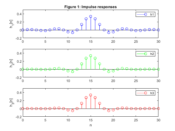
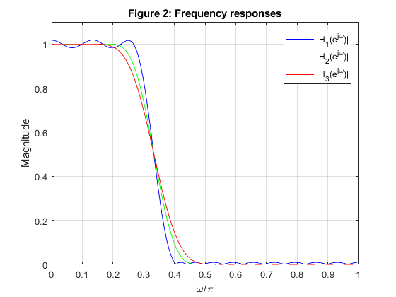
Use the MATLAB function firnyquist to design linear-phase FIR Lth-band filters of the length N =31, with L = 3 and with the roll-off factors: ρ = 0.2, 0.4, and 0.6.
Plot the impulse responses and the magnitude responses for all designs.

Used functions: firnyquist (DSP System Toolbox), freqz (Signal Processing Toolbox)

close all, clear all
N =31;                                    % Filter length
Nord = N-1;                               % Filter order
L = 3;
ro1 = 0.2;                                % Roll-off factor
h1 = firnyquist(Nord,L,ro1);              % Filter design
ro2 = 0.4;                                % Roll-off factor
h2 = firnyquist(Nord,L,ro2);              % Filter design
ro3 = 0.6;                                % Roll-off factor
h3 = firnyquist(Nord,L,ro3); % filter design
figure (1)
subplot(3,1,1)
stem(0:N-1,h1,'b'), axis([0,30,-0.2,0.5]), ylabel('h_1[n]')
title('Figure 1: Impulse responses')
legend('h1')
subplot(3,1,2)
stem(0:N-1,h2,'g'), axis([0,30,-0.2,0.5]), ylabel('h_2[n]')
legend('h2')
subplot(3,1,3)
stem(0:N-1,h3,'r'), axis([0,30,-0.2,0.5]), xlabel('n'), ylabel('h_3[n]')
legend('h3')
% Computing frequency responses
[H1,f] = freqz(h1,1,256,2);
[H2,f] = freqz(h2,1,256,2);
[H3,f] = freqz(h3,1,256,2);
figure (2)
plot(f,abs(H1),'b',f,abs(H2),'g',f,abs(H3),'r'), grid
title ('Figure 2: Frequency responses')
axis([0,1,0,1.1]),xlabel('\omega/\pi'), ylabel('Magnitude')
legend('|H_1(e^j^\omega)|','|H_2(e^j^\omega)|','|H_3(e^j^\omega)|')

Exercise 7.2

Use the Lth-band filters from the MATLAB Exercise 7.1 for interpolation.
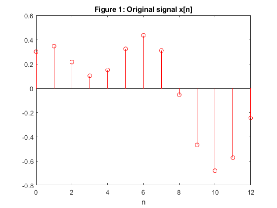
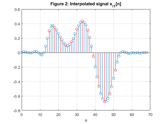
Generate the original signal {x[n]} according to your own choice, and then interpolate this signal by-the-factor-of-3.
Perform the interpolation using three distinct interpolation filters from Exercise 7.1.
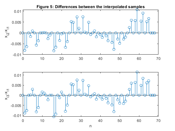
Compare and comment on the results.

Used functions: firnyquist (DSP System Toolbox), upsample (Signal Processing Toolbox)

close all, clear all
% Computing the coefficients of the 3 Lth-band filters of Example 7.1:
N =31;                                  % Filter length
Nord = N-1;                             % Filter order
L = 3;
ro1 = 0.2;                              % Roll-off factor
h1 = firnyquist(Nord,L,ro1); % filter design
ro2 = 0.4;                              % Roll-off factor
h2 = firnyquist(Nord,L,ro2);            % Filter design
ro3 = 0.6;  % roll-off factor
h3 = firnyquist(Nord,L,ro3);            % Filter design

% Generating the signal x[n]
n = 0:12;
x = 0.4*sin(pi*0.14*n)+0.3*cos(pi*0.3*n);
figure (1)
stem(n,x,'r'), xlabel('n')
title('Figure 1: Original signal x[n]')

% Interpolation: upsampling and filtering
xi1 = 3*conv(h1,upsample(x,3));
xi2 = 3*conv(h2,upsample(x,3));
xi3 = 3*conv(h3,upsample(x,3));

figure (2)
stem(0:length(xi1)-1,xi1)
hold on
stem(15+3*n,x,'r'), grid
xlabel('n'), title('Figure 2: Interpolated signal x_i_1[n]')

figure (3)
stem(0:length(xi2)-1,xi2)
hold on
stem(15+3*n,x,'r'), grid
xlabel('n'), title('Figure 3: Interpolated signal x_i_2[n]')

figure (4)
stem(0:length(xi3)-1,xi3)
hold on
stem(15+3*n,x,'r'), grid
xlabel('n'), title('Figure 4: Interpolated signal x_i_3[n]')

% COMMENTS
% 1. The every third sample value in the interpolated sequences xi1, xi2, and xi3
% retains the corresponding sample value of the original sequence x[n], see
% Figures 2-4 where x[n] is delayed for (N-1)/2 = 15 samples.
% 2. The differences between the interpolated sequences xi1, xi2, and xi3
% are very small, see Figure 5.
figure (5)
subplot(2,1,1)
stem(0:length(xi2)-1,xi2-xi1)
ylabel('x_i_2-x_i_1')
title('Figure 5: Differences between the interpolated samples')
subplot(2,1,2)
stem(0:length(xi3)-1,xi3-xi1)
xlabel('n'), ylabel('x_i_3-x_i_1')

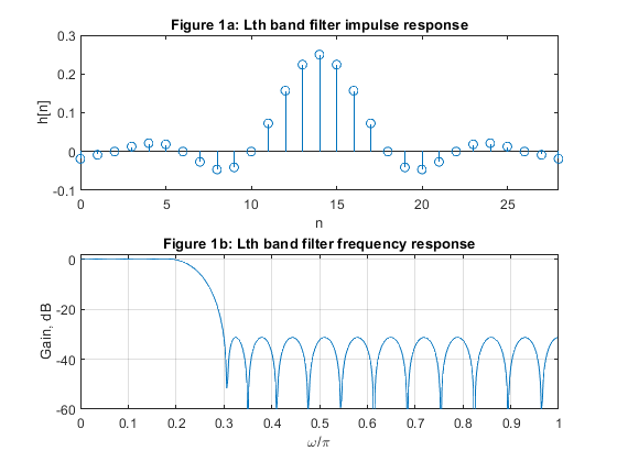
Exercise 7.3

Design a linear-phase Lth-band FIR filter with the following parameters: N = 29, L =4, ρ = 0.2.
Construct the polyphase factor-of-4 decimator using the efficient configuration of Figure 4.8 from the book.
Which one of four polyphase subfilters reduces to a constant?
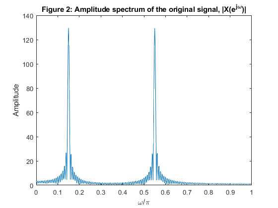
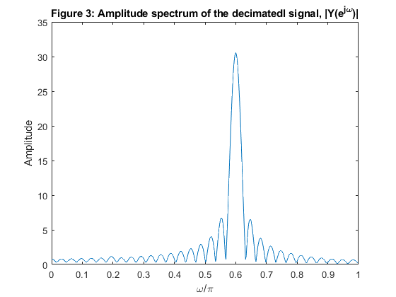
Generate a signal to your own choice and decimate this signal by M = 4.
Plot the impulse response and the magnitude response of the filter.
Plot the signal spectrum before and after decimation.

Figure 4.8 (from the book): Commutative polyphase structure of a decimator

Used functions: firnyquist (DSP System Toolbox), downsample, freqz (Signal Processing Toolbox)

close all, clear all
% Computing the coefficients of the Lth-band decimation filter:
N =29;                                           % Filter length
Nord = N-1;                                      % Filter order
L = 4;
ro = 0.2;                                        % Roll-off factor
h = firnyquist(Nord,L,ro);                       % Filter design
[H,f] = freqz(h,1,500,2);                        % Computing the frequency response

figure (1)
subplot(2,1,1)
stem(0:N-1,h),xlabel('n'),ylabel('h[n]')
title('Figure 1a: Lth band filter impulse response')
axis([0,N-1,-0.1,0.3])
subplot(2,1,2)
plot(f,20*log10(abs(H))), xlabel('\omega/\pi'),ylabel('Gain, dB')
title('Figure 1b: Lth band filter frequency response')
axis([0,1,-60,2]), grid

% Polyphase components of the decimation filter h[n]
e0 = downsample(h,4,0);
e1 = downsample(h,4,1);
e2 = [0,0,0,0.25,0,0,0];         % This polyphase component reduces to the delay z^(-3) multiplied by 0.25.
e3 = downsample(h,4,3);

% Generating the original signal x[n]
n = 0:255;
x = cos(pi*0.15*n)+cos(pi*0.55*n);
[X,f] = freqz(x,1,500,2);
figure (2)
plot(f,abs(X))
xlabel('\omega/\pi'),ylabel('Amplitude')
title('Figure 2: Amplitude spectrum of the original signal, |X(e^j^\omega)|')

% Polyphase downsampling of the original signal
x0 = [x(1:4:256),0]; x1 = [0,x(4:4:256)]; x2 =[0,x(3:4:256)]; x3 = [0,x(2:4:256)];

% Polyphase filtering
y0 = filter(e0,1,x0);
y1 = filter(e1,1,x1);
y2 = 0.25*[0,0,0,x2(1:length(x2)-3)];
y3 = filter(e3,1,x3);

% Decimated signal y[n]
y = y0+y1+y2+y3;
[Y,fd] = freqz(y,1,500,2);
figure (3)
plot(fd,abs(Y))
xlabel('\omega/\pi'),ylabel('Amplitude')
title('Figure 3: Amplitude spectrum of the decimatedl signal, |Y(e^j^\omega)|')

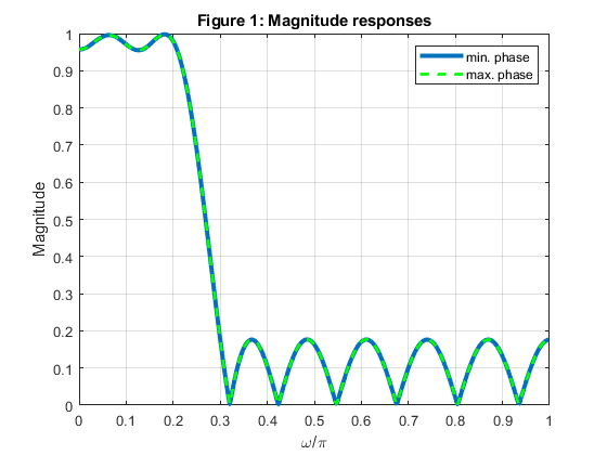
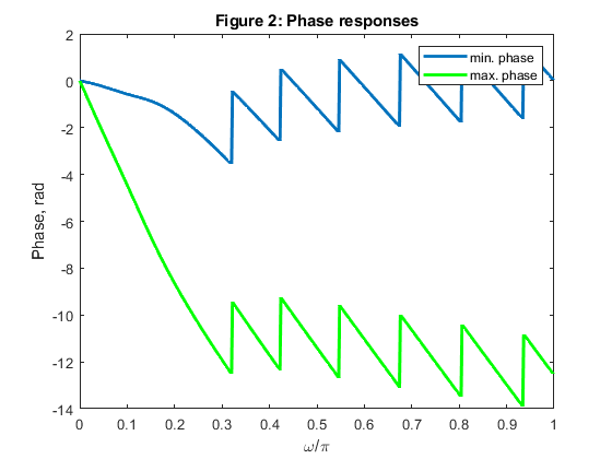
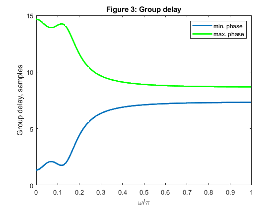
Exercise 7.4

Design the minim-phase and the maximum-phase Lth-band FIR filters with the following design parameters: N_ord = 17, L = 4, and ρ = 0.2.
Plot magnitude, phase, and group delay responses for both filters.
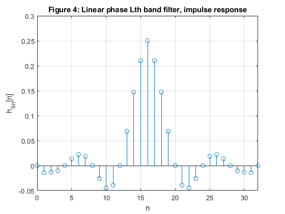
Compose the linear-phase filter by convolving the impulse responses of the minimum-phase and the maximum phase filters.
Plot the impulse response of the linear-phase filter and verify the zero-crossing positions.
Comment on the results.

Used functions: firnyquist (DSP System Toolbox), freqz, grpdelay (Signal Processing Toolbox)

close all, clear all
N =17;                                           % Filter length
Nord = N-1;                                      % Filter order
L = 4;
ro = 0.2;                                        % Roll-off factor
% Computing the coefficients of the Lth-band minimum phase filter:
h_min = firnyquist(Nord,L,ro,'minphase');        % Filter design
[H_min,f] = freqz(h_min,1,500,2); % computing the frequency response
figure (1)
plot(f,abs(H_min),'Linewidth',3), xlabel('\omega/\pi'),ylabel('Magnitude')
title('Figure 1: Magnitude responses'), grid
hold on
% Computing the coefficients of the Lth-band maximunm phase filter:
h_max = fliplr(h_min);                           % Filter design
[H_max,f] = freqz(h_max,1,500,2);                % Computing the frequency response
figure (1)
plot(f,abs(H_max),'--g','Linewidth',2)
legend('min. phase','max. phase')

figure (2)
plot(f,unwrap(angle(H_min)),f,unwrap(angle(H_max)),'g','Linewidth',2)
xlabel('\omega/\pi'),ylabel('Phase, rad'), title('Figure 2: Phase responses')
legend('min. phase','max. phase')

[gd_min,f] = grpdelay(h_min,1,500,2);
[gd_max,f] = grpdelay(h_max,1,500,2);

figure (3)
plot(f,gd_min,f,gd_max,'g','Linewidth',2)
xlabel('\omega/\pi'),ylabel('Group delay, samples'), title('Figure 3: Group delay')
legend('min. phase','max. phase')

% Composing linear phase filter h_lin
h_lin = conv(h_min,h_max);
figure (4)
stem(0:length(h_lin)-1,h_lin), grid
xlabel('n'),ylabel('h_l_i_n[n]')
title('Figure 4: Linear phase Lth band filter, impulse response')
axis([0,length(h_lin)-1,-0.05,0.3])

% COMMENTS:
% 1. Magnitude responses of minimum-phase and maximum phase filters are
% identical, see Figure 1.
% 2. Difference in phase responses of two filters, H_min and H_max are
% illustrated in Figure 2.
% 3. Figure 3 illustrates the group dalay properties of  H_min and H_max:
% filter H_max exhibits higher delay for all frequencies.
% 4. The convolution of the impulse responses of minimum-phase and maximum-
% phase Lth-band filters (h_min and h_max) results in a linear-phase Lth-band filter.
% For L=4, every 4th sample in h_lin is zero-valued (excluding the central sample), see Figure 4.

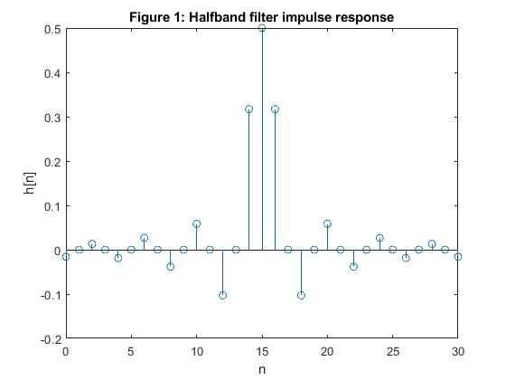
Exercise 7.5

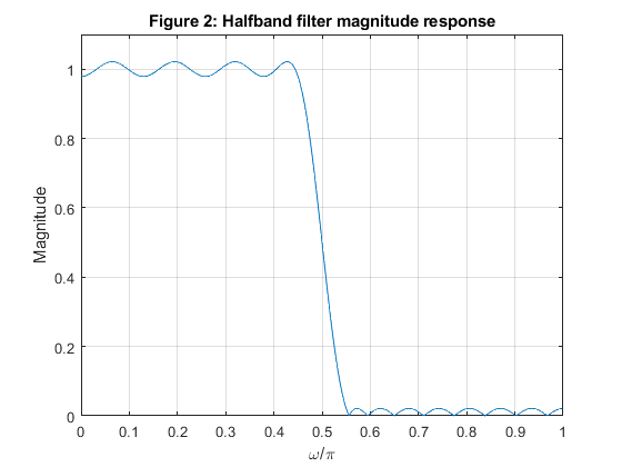
Design an equiripple linear-phase halfband filter of the length N = 31, and the passband edge frequency at ω_p = 0.45π.
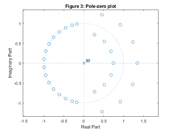
Compute and plot the impulse response, magnitude response and pole-zero locations in the z-plane.

Used functions: firhalfband (DSP System Toolbox), freqz, zplane (Signal Processing Toolbox)

close all, clear all
N = 31;                                  % Filter lengh
fp = 0.45;                               % Passband edge frequency
Nord = N-1;
h = firhalfband(Nord,fp);                % Halfband filter design
figure (1)
stem(0:N-1,h)
xlabel('n'), ylabel('h[n]'), title('Figure 1: Halfband filter impulse response')
[H,f] = freqz(h,1,500,2);                % Halfband filter frequency response
figure (2)
plot(f,abs(H))
xlabel('\omega/\pi'),ylabel('Magnitude'), grid
title('Figure 2: Halfband filter magnitude response')
axis([0,1,0,1.1])
figure(3)
zplane(h,1)
title('Figure 3: Pole-zero plot')

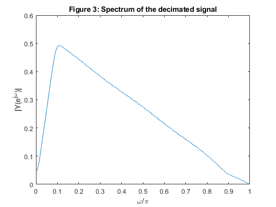
Exercise 7.6

Develop the efficient interpolator structure based on the linear-phase FIR half-band filter.
Modify program demo_7_1 (from the book) to perform the interpolation-by-2.
For the input signal use the decimated signal obtained in demo_7_1.

Solution of the Exercise consists of two steps:
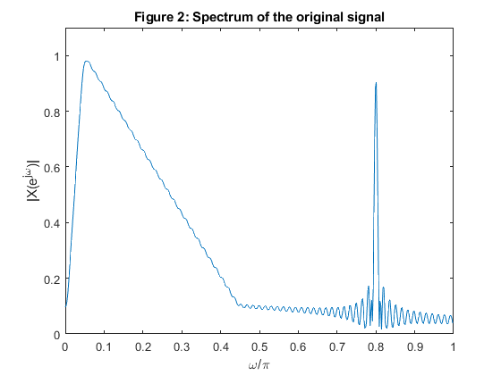
STEP 1: Run program demo_7_1.m to compute signal {y[n]} to be interpolated in STEP 2.
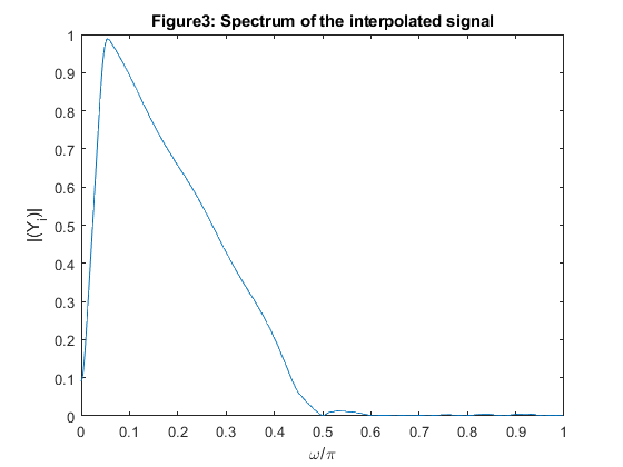
STEP 2: Based on the implementation structure depicted in Figure 1b develop MATLAB code for interpolation-by-two.

Figure 1: Efficient implementation structure of the factor-of-2 interpolator based on the linear-phase FIR halfband filter.
(a) Polyphase configuration. (b) Implementation scheme for N = 11.

Used functions: firhalfband (DSP System Toolbox), freqz (Signal Processing Toolbox)

clear all, close all
% STEP 1
% Program demo_7_1
%
h = firhalfband(22,0.4);                   % FIR filter design
% Generation of the input signal
F = [0,0.05,0.45,1]; A = [0,1,0.1,0.05];
x1 = fir2(256,F,A); x2 = sin(2*pi*(0:256)*0.4)/150;
x = x1 + x2;
[X,f] = freqz(x,1,512,2);                 % Spectrum of the original signal
figure (2)
plot(f,abs(X(1:512))), xlabel('\omega/\pi'),ylabel('|X(e^{j\omega})|')
title('Figure 2: Spectrum of the original signal')
axis([0,1,0,1.1])

% Polyphase decomposition
e0 = h(1:2:(length(h)-1)/2);

% Setting the initial states
xk = zeros(size(1:(length(h)+1)/2));

% Decimation
rot = 0; % Initial swithch position
y = [];
for n=1:length(x)
xn = x(n);

if rot==0 ss=1;
    pro = xn*e0;
    xk = [pro+xk(1:length(xk)/2),fliplr(pro) + xk((length(xk)/2+1):length(xk))];
    yn = xk(length(xk));
    y = [yn,y];
    xk = [0,xk(1:length(xk)-1)];
else
end
if rot==1 ss=0;
    xk(length(xk)/2+1) = 0.5*xn + xk(length(xk)/2+1);
else
end
rot=ss;
end

Y = freqz(y,1,512,2);                     % Spectrum of the decimated signal
figure (3)
plot(f,abs(Y(1:512))), xlabel('\omega/\pi'),ylabel('|Y(e^{j\omega})|')
title('Figure 3: Spectrum of the decimated signal')
axis([0,1,0,0.6])
%
% STEP 2
% Interpolation according to Figure 1
yi=[];
xk=zeros(size(1:(length(h)+1)/2));
rot=0;
k=1;
for n=1:length(y)*2-1
    xn=y(k);
    if k==1,  xk=[xn,xk(1:length(xk)-1)];
    else
    end

if rot==0 ss=1;
    yn=2*sum((xk(1:length(xk)/2)+fliplr(xk(length(xk)/2+1:length(xk)))).*e0);
    yi=[yi,yn];
else
end
if rot==1 ss=0;
    yi=[yi,xk(length(xk)/2)];
    if k>1  xk=[xn,xk(1:length(xk)-1)];
else
end
    k=k+1;
else
end

rot=ss;
end

[Yi,f]=freqz(yi,1,512,2);                % Spectrum of the interpolated signal
figure(4)
plot(f,abs(Yi));title('Figure3: Spectrum of the interpolated signal')
xlabel('\omega/\pi'),ylabel('|(Y_i)|')

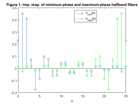
Exercise 7.7

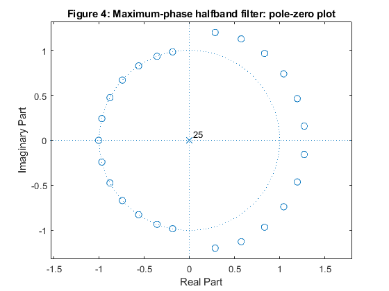
Design the minimum-phase and maximum phase halfband FIR filters of the order N_ord = 25.
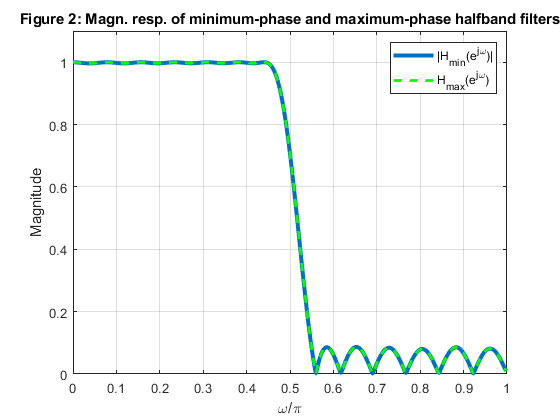
Compute and plot the magnitude response and the zero-pole plot for both filters.
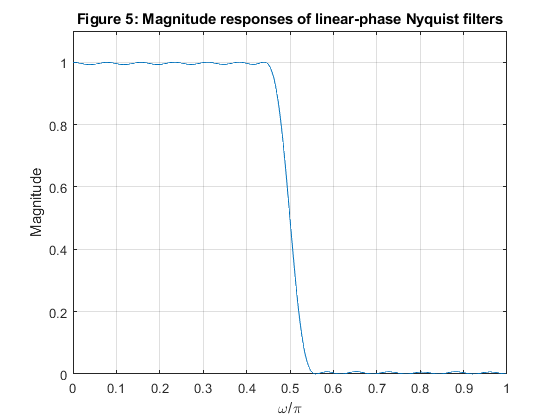
Compute the impulse response of the linear-phase Nyquist filter by convolving the impulse responses of the minimum-phase and the maximum-phase filters.
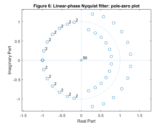
Compute and plot the magnitude response and the zero-pole plot of the linear-phase Nyquist filter.
Comment on the results.

Used functions: firhalfband (DSP System Toolbox), freqz (Signal Processing Toolbox)

close all, clear all
Nord = 25;                                % Filter lengh
fp = 0.45;                                % We chose the passband edge frequency
h_min = firhalfband(Nord,fp,'minphase');  % Minimum-phase halfband filter design
h_max = fliplr(h_min);
figure (1)
stem(0:Nord,h_min)
hold on
stem(0:Nord,h_max,'gs')
xlabel('n'),  title('Figure 1: Imp. resp. of minimum-phase and maximum-phase halfband filters')
legend('h_m_i_n[n]','h_m_a_x[n]','Location','best')
[H_min,f] = freqz(h_min,1,500,2);        % Minimum-phase halfband filter frequency response
[H_max,f] = freqz(h_max,1,500,2);        % Maximum-phase halfband filter frequency response
figure (2)
plot(f,abs(H_min),'Linewidth',3)
hold on
plot(f,abs(H_max),'--g','Linewidth',2)
xlabel('\omega/\pi'),ylabel('Magnitude'), grid
title('Figure 2: Magn. resp. of minimum-phase and maximum-phase halfband filters')
legend('|H_m_i_n(e^j^\omega)|','H_m_a_x(e^j^\omega)')
axis([0,1,0,1.1])
figure(3)
zplane(h_min,1)
title('Figure 3: Minimum-phase halfband filter: pole-zero plot')
figure (4)
zplane(h_max,1)
title('Figure 4: Maximum-phase halfband filter: pole-zero plot')
% Linear-phase Niquist filter
h = conv(h_min,h_max);
[H,f] = freqz(h,1,500,2);
figure (5)
plot(f,abs(H))
xlabel('\omega/\pi'),ylabel('Magnitude'), grid
title('Figure 5: Magnitude responses of linear-phase Nyquist filters')
axis([0,1,0,1.1])
figure (6)
zplane(h,1)
title('Figure 6: Linear-phase Nyquist filter: pole-zero plot')

% COMMENTS:
% 1. Impulse response of the maximum-phase halfband filter is obtained by
% inverting the impulse response of minimum-phase halfband filter, see
% Figure 1.
% 2. Magnitude responses of minimum-phase and maximum phase filters are
% identical, see Figure 2.
% 3. The transfer function zeros of the minimum-phase filter are placed
% inside the unit circle or on the unit circle, see Figure 3.
% 4. The transfer function zeros of the maximum-phase filter are placed
% outside the unit circle or on the unit circle, see Figure 4.
% 5. Convolution of the impulse responses of the minimum-phase and maximum-
% phase halfband filters (h_min and h_max) results in the linear-phase
% halfband Niqyist filter. Figure 5 illustrates the double zeros of the
% filter magnitude response.
% 6. The transfer function zeros of the resulting linear-phase halfband filter,
% which are placed on the unit circle, are double zeros. The remaining zeros
% are symmetric in the respect to the unit circle, see Figure 6.

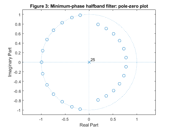
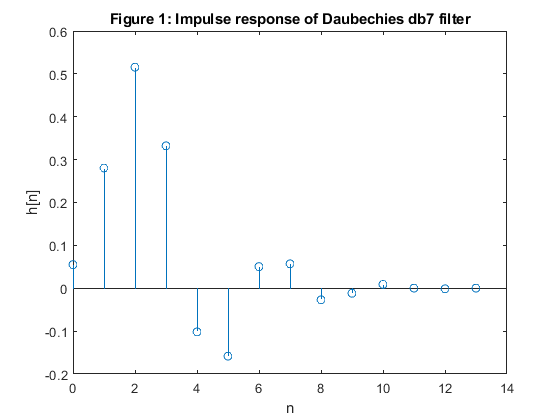
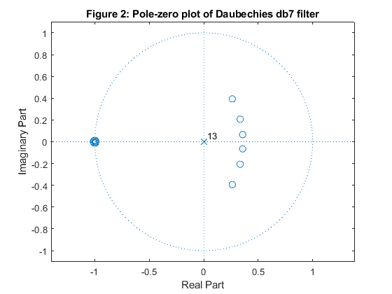
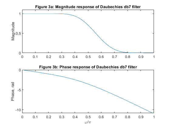
Exercise 7.8

Use the MATLAB function dbwavf from the Wavelet Toolbox to design Daubeschies filter db7.
Plot the impulse response, zero-pole plot, magnitude and phase responses.

Used functions: dbwavf (Wavelet Toolbox), freqz (Signal Processing Toolbox)

close all, clear all
wname = 'db7';                       % Set Daubechies wavelet name
h = dbwavf(wname);                   % Filter desogn
figure (1)
stem(0:length(h)-1,h)
xlabel('n'), ylabel('h[n]')
title('Figure 1: Impulse response of Daubechies db7 filter')
figure (2)
zplane(h,1)
title('Figure 2: Pole-zero plot of Daubechies db7 filter')
figure (3)
[H,f] = freqz(h,1,200,2);
subplot(2,1,1)
plot(f,abs(H)),axis([0,1,0,1.1]), ylabel('Magnitude')
title('Figure 3a: Magnitude response of Daubechies db7 filter')
subplot(2,1,2)
plot(f,unwrap(angle(H))), xlabel('\omega/\pi'),ylabel('Phase, rad')
title('Figure 3b: Phase response of Daubechies db7 filter')

Exercise 7.9

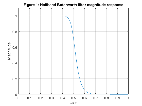
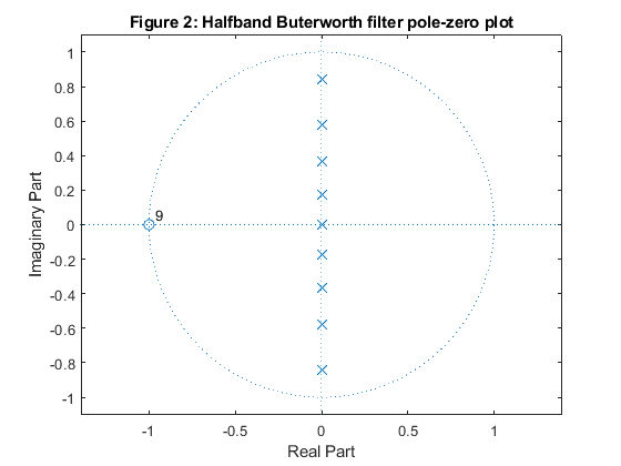
Design the 9th-order Butterworth halfband filter. Compute and plot the magnitude response and display the pole-zero plot of the filter.
Consider the implementation structure based on the parallel connection of two allpass subfilters A₀(z) and A₁(z) according to equations (7.38) – (7.40) from the book:

H(z)=(A₀(z)+z^{- 1}A₁(z))/2, (7.38)

Eq. 7.39 left and Eq. 7.39 right . (7.39)

β_l=(r_l)², with β_l< β _l+1, l=2, 3, …, (N+1)/2. (7.40)

Determine the constants in the second-order sections of A₀(z) and A₁(z).

Used functions: butter, freqz (Signal Processing Toolbox)

close all, clear all
N = 9; % filter order
[b,a] = butter(N,0.5);              % Butterworth filter design: computing the transfer function constants
[z,p,k] = butter(N,0.5);            % Butterworth filter design: computing the poles and zeros
[H,f] = freqz(b,a,500,2);           % Computing the frequency response
Mag = abs(H);                       % Computing the magnitude response
figure (1)
plot(f,Mag), xlabel('\omega/\pi'), ylabel('Magnitude')
axis([0,1,0,1.1]), grid
title('Figure 1: Halfband Buterworth filter magnitude response')
figure (2)
zplane(z,p)
title('Figure 2: Halfband Buterworth filter pole-zero plot')

% Implementation based on the parallel connection of two allpass subfilters A0(z) and A1(z)

pp = sort(abs(p).^2);
beta_HB = pp(2:2:length(pp));       % Constants of the halfband filter H(z)
beta_HB_A0 = beta_HB(1:2:4);        % Constants in the second order sections of A0(z)
beta_HB_A1 = beta_HB(2:2:4);        % Constants in the second order sections of A1(z)
disp(['Constants of the Butterworth halfband filter H(z): ', num2str(beta_HB')]);
disp(['Constants in the second-order sections of A0(z):   ', num2str(beta_HB_A0')]);
disp(['Constants in the second-order sections of A1(z):   ', num2str(beta_HB_A1')]);

Constants of the Butterworth halfband filter H(z): 0.031091     0.13247     0.33333     0.70409
Constants in the second-order sections of A0(z):   0.031091     0.33333
Constants in the second-order sections of A1(z):   0.13247     0.70409

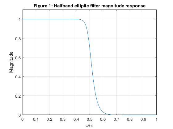
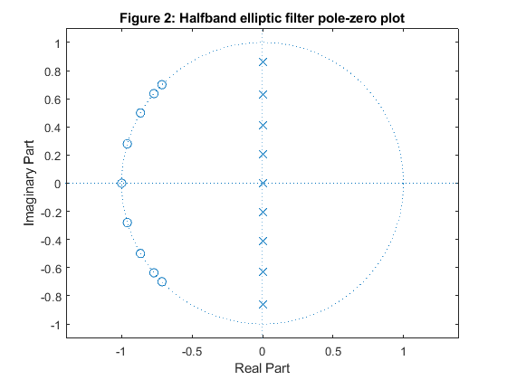
Exercise 7.10

Use the program halfbandiir given in Appendix A to design the 9th-order elliptic halfband filter.
Compute and plot the magnitude response and display the pole-zero plot of the filter.
Consider the implementation structure based on the parallel connection of two allpass subfilters A₀(z) and A₁(z) according to (7.38) – (7.40) from the book:

H(z)=(A₀(z)+z^{- 1}A₁(z))/2, (7.38)

Eq. 7.39 left and Eq. 7.39 right . (7.39)

β_l=(r_l)², with β_l< β _l+1, l=2, 3, …, (N+1)/2. (7.40)

Determine the constants in the second-order sections of A₀(z) and A₁(z).

Used functions: freqz (Signal Processing Toolbox), halfbandiir, (Appendix)

close all, clear all
N = 9; % filter order
[b,a,z,p,k] = halfbandiir(N,0.5/2); % Elliptic filter design: computing the transfer function constants

[H,f] = freqz(b,a,500,2);           % Computing the frequency response
Mag = abs(H);                       % Computing the magnitude response
figure (1)
plot(f,Mag), xlabel('\omega/\pi'), ylabel('Magnitude')
axis([0,1,0,1.1]), grid
title('Figure 1: Halfband elliptic filter magnitude response')
figure (2)
zplane(z,p)
title('Figure 2: Halfband elliptic filter pole-zero plot')

% Implementation based on the parallel connection of two allpass subfilters A0(z) and A1(z)
pp = sort(abs(p).^2);
beta_HB = pp(2:2:length(pp));      % Constants of the halfband filter
beta_HB_A0 = beta_HB(1:2:4);       % Constants in the second order sections of A0(z)
beta_HB_A1 = beta_HB(2:2:4);       % Constants in the second order sections of A1(z)
disp(['Constants of the elliptic halfband filter H(z):  ', num2str(beta_HB')]);
disp(['Constants in the second-order sections of A0(z): ', num2str(beta_HB_A0')]);
disp(['Constants in the second-order sections of A1(z): ', num2str(beta_HB_A1')]);

Constants of the elliptic halfband filter H(z):  0.042455     0.17074     0.39332     0.74571
Constants in the second-order sections of A0(z): 0.042455     0.39332
Constants in the second-order sections of A1(z): 0.17074     0.74571