Multirate Filtering for Digital Signal Processing: MATLAB® Applications, Chapter VI: Sampling Rate Conversion by a Fractional Factor - Exercises
Contents
Exercise 6.1
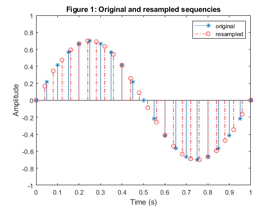
Modify program demo_6_1 to convert the sampling
frequency by the factor 5/4.
Plot the samples of input and the samples of the output signals.
Used function: resample (Signal Processing Toolbox)
clear all, close all
% Sampling rate conversion by L/M = 5/4
Fx = 20;                                            % Original sampling frequency in Hz
Tx=1/Fx;                                            % Original sampling period in seconds
tx = 0:Tx:1;                                        % Time vector tx
x = 0.7*sin(2*pi*tx);                               % Original sequence
y = resample(x,5,4);                                % Re-sampling
ty = (0:(length(y)-1))*4*Tx/5;                      % New time vector ty
figure (1)
stem(tx,x,'*')
hold on
stem(ty,y,'-.r')
title('Figure 1: Original and resampled sequencies')
legend('original','resampled','Location','northeast')
xlabel('Time (s)'), ylabel('Amplitude'), axis([0,1,-1,1])
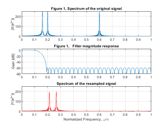
Exercise 6.2
Use the MATLAB function upfirdn to convert the sampling rate by the factor L/M = 3/4:
a) Design an optimal FIR filter of the length
N = 64 to approximate the ideal specifications as given in
(6.2).
 . (6.2)
b) Generate 512 samples of the input signal {x[n]} given by
{x[n]}] = sin(2π0.08n) +
sin(2π0.1n) + sin(2π0.3n).
Compute the samples of the resampled signal
{y[n]}.
c) Plot the frequency response of the filter, and the spectrum of the signal {x[n]},
and that of the resampled signal {y[n]}.
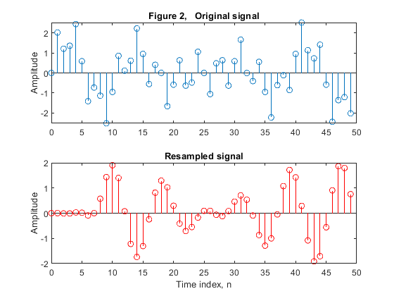
Plot the first 50 samples of the original signal,
and the first 50 samples of the resampled signal.
Comment on the results.
Used functions: upfirdn, freqz (Signal Processing Toolbox), firgr (DSP System Toolbox)
clear all, close all
L=3; M=4;

% Input signal x[n]
n = 0:511;                                              % Time index
x1 = sin(2*pi*0.08*n); x2 = sin(2*pi*0.1*n);
x3 = sin(2*pi*0.3*n);
x = x1 + x2 + x3;                                        % Generating the original signal {x[n]}
[X,f] = freqz(x,1,1028,2);                               % Spectrum of the original signal
subplot(3,1,1),  plot(f,abs(X)), grid on
title('Figure 1, Spectrum of the original signal')
ylabel('|X(e^j^\omega)|'), axis([0,1,0,250])

% Lowpass filter specifications: to pass components x1 and x2, and to
% suppress component x3:  Fp>0.2/L;  Fs<0.6/L
N = 64;                                                 % Filter length
Fp = 0.25/3; Fs = 0.19; amp =  [1,1,0,0];               % Setting filter design parameters
h = firgr(N-1,[0,Fp,Fs,1],amp);                         % Filter design
[H,f]=freqz(h,1,512,2);                               % Computing frequency response
figure (1)
subplot(3,1,2),  plot(f,20*log10(abs(H))), grid on
title('Figure 1,   Filter magnitude response')
ylabel('Gain [dB]'),axis([0,1,-80,5])

% Computing resampled signal y[n]
y = upfirdn(x,L*h,L,M);                                 % Computing the resampled signal {y[n]}
[Y,f] = freqz(y,1,1028,2);                              % Spectrum of the signal {y[n]}
subplot(3,1,3),  plot(f,abs(Y),'r'), grid on
title('Spectrum of the resampled signal')
xlabel('Normalized Frequency, \omega/\pi'), ylabel('|Y(e^j^\omega)|')
axis([0,1,0,250])

figure (2)
n=0:49;
subplot(2,1,1)
stem(n,x(1:50)),ylabel('Amplitude'), title('Figure 2,   Original signal')
subplot(2,1,2)
stem(n,y(1:50),'r'), title('Resampled signal')
xlabel('Time index, n'),ylabel('Amplitude')
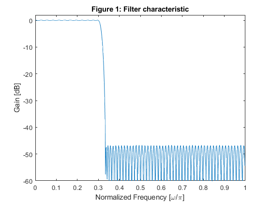
Exercise 6.3
Modify program demo_6_2 to perform the sampling rate alteration with
the fractional factor L/M = 2/3.
The implementation structure is given in Figure 6.7.
Structure of the efficient sampling-rate converter for L/M = 2/3.
(Figure 6.7 of the book).
Used functions: fir2, freqz, (Signal Processing Toolbox), firgr (DSP System Toolbox)
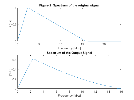
clear all, close all
% Lowpass filter design
N = 144;                                                % FIR filter length
Fp = 0.9/3; Fs = 1/3; amp =  [1,1,0,0];                 % Setting filter design parameters
h = firgr(N-1,[0,Fp,Fs,1], [1,1,0,0]);                  % Filter design
[H,f]=freqz(h,1,512,2);                                 % Filter frequency response
figure (1)
plot(f,20*log10(abs(H)))
xlabel('Normalized Frequency [\omega/\pi]'),  ylabel('Gain [dB]')
title('Figure 1: Filter characteristic')
axis([0,1,-60,2])

% Generating the input signal {x[n]}
L=2; M=3;
Fx = 48000; Fy = 32000;
F = [0,0.1,0.66,1]; m = [0,1,0,0];                      % Setting the input parameters for fir2
x = fir2(255,F,m);                                      % Generating the original signal {x[n]}
[X,f] = freqz(x,1,512,Fx);                              % Spectrum of the original signal
figure (2)
subplot(2,1,1),  plot(f/1000,abs(X))
xlabel('Frequency [kHz]'), ylabel('|X(F)|'), axis([0,24,0,1])
title('Figure 2, Spectrum of the original signal')

% Polyphase decomposition
e0 = h(1:2:length(h)); e1 = h(2:2:length(h));
E0=reshape(e0,3,length(e0)/3);
E1=reshape(e0,3,length(e1)/3);

% Down-sampling
u1 = x;
u0 = [0,x(1:length(x)-1)];
u00d = u0(1:3:length(u0));
u01d = [0,u0(3:3:length(u0))];
u02d = [0,u0(2:3:length(u0))];
u10d = u1(1:3:length(u1));
u11d = [0,u1(3:3:length(u1))];
u12d = [0,u1(2:3:length(u1))];

% Polyphase filtering
x00 = filter(2*E0(1,:),1,u00d);
x01 = filter(2*E0(2,:),1,u01d);
x02 = filter(2*E0(3,:),1,u02d);
x10 = filter(2*E1(1,:),1,u10d);
x11 = filter(2*E1(2,:),1,u11d);
x12 = filter(2*E1(3,:),1,u12d);

yy0=x00+x01+x02;
yy1=x10+x11+x12;

y0ii=zeros(1,L*length(yy0));
y1ii=zeros(1,L*length(yy1));
y0ii(1:L:length(y0ii))=yy0;                            % Up-sampled signal
y1ii(1:L:length(y1ii))=yy1;                            % Up-sampled signal

y1 = [0,(y1ii(1:(length(y1ii)-1)))];

y = y0ii+y1;                                             % Output signal
[Y,f] = freqz(y,1,512,Fy);                               % Frequency response of the output signal
subplot(2,1,2), plot(f/1000,abs(Y))
xlabel('Frequency [kHz]'), ylabel('|Y(F)|'), axis([0,16,0,0.7])
title('Spectrum of the Output Signal')
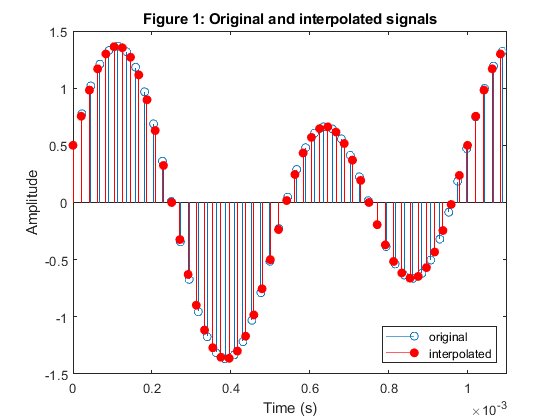
Exercise 6.4
Use the MATLAB function interp1 with the option spline to convert the sampling rate of the signal x(t)=sin(2*pi*2000*t)+0.5*cos(2*pi*1000*t) from 44.1 kHz to 48 kHz.
clear all; close all;
M = 147; L = 160;                                        % Interpolation/decimation factors.

Fx = 44.1e3;                                             % Sampling frequency of the original signal: 44.1kHz
Fy= Fx*L/M;                                              % Sampling frequency of the interpolated signal
n = 0:99;                                                % Time index
tx = n/Fx;                                               % Time vector tx
ty = n/Fy;                                               % New time vector ty
ny = n*L/M;
x = sin(2*pi*2000*tx)+0.5*cos(2*pi*1000*tx);             % Original signal {x{n*Tx)}
y = interp1(tx,x,ty,'spline');                           % Interpolated signal {y{n*Ty)}

figure (1)
stem(tx(1:49),x(1:49)); hold on
stem(ty(1:54),y(1:54),'r','filled');
xlabel('Time (s)');ylabel('Amplitude');axis([0,1.1e-3,-1.5,1.5])
title('Figure 1: Original and interpolated signals')
legend('original','interpolated','Location','southeast')
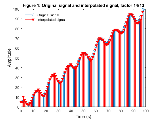
Exercise 6.5
Modify program demo_6_3 (pagees 193-194 in the book) to perform the interpolation by a fractional factor 14/13 using the cubic Lagrange polynomials and the Farrow structure.
clear all, close all
% Sampling-rate alteration by the fractional factor R = 14/13

% Generating the input signal {x[n]}
n = -2:100;
f1 = 0.1; f2 = 0.16;
x = n+2*sin(pi*f1*n)+5*cos(pi*f2*n);                     % Original signal {x[n]}

% Defining fractional intervals for sampling rate alteration by 16/15
R = 14/13;                                               %  Re-sampling factor
s = 1:13;
mu = [0,1-(1-1/R)*s];
mu = repmat(mu,1,8);                                     % Vector of fractional intervals

% Farrow filter, coefficients:
C0 = [1/6,-1/2,1/2,-1/6];                                % Vector of Lagrange coefficients for C_0(k)
C1 = [0,1/2,-1,1/2];                                     % Vector of Lagrange coefficients for C_1(k)
C2 = ([-1/6,1,-1/2,-1/3]);                               % Vector of Lagrange coefficients for C_2(k)
C3 = [0,0,1];                                            % Vector of Lagrange coefficients for C_3(k)

% Farrow filter, initial states:
xs0 = [0,0,0]; xs1 = [0,0,0]; xs2 = [0,0,0]; xs3 = [0,0];

% Farrow filtering:
l=1;
for n=1:1:100
    xnl = x(n+2);
[v0,xs0] = filter(C0,1,xnl,xs0);
[v1,xs1] = filter(C1,1,xnl,xs1);
[v2,xs2] = filter(C2,1,xnl,xs2);
[v3,xs3] = filter(C3,1,xnl,xs3);
if mu(l)==0
     y(l) = ((v0*mu(l)+v1)*mu(l)+v2)*mu(l)+x(n+2);
    y(l+1) = ((v0*mu(l+1)+v1)*mu(l+1)+v2)*mu(l+1)+x(n+2);
    l = l + 2;
else
    y(l) = ((v0*mu(l)+v1)*mu(l)+v2)*mu(l)+x(n+2);
    l = l + 1;
end
end
figure (1)
tx=0:length(x)-5;                                        % Time vector tx
ty=(0:length(y)-3)*13/14;                                % New time vector ty
stem(tx,x(3:length(x)-2))
hold on
stem(ty,y(1:length(y)-2),'rv','filled')
legend('Original signal','Interpolated signal','Location','northwest')
xlabel('Time (s)'), ylabel('Amplitude'),
title('Figure 1: Original signal and interpolated signal, factor 14/13')
Exercise 6.6
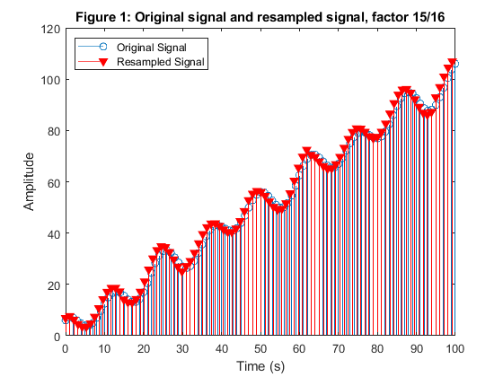
Based on the program demo_6_3 (pagees 193-194 in the book), develop the program which simulates the factor-of-15/16-decimator using the cubic Lagrange polynomials and the Farrow structure.
clear all, close all
% Generating the input signal x[n]
n = -2:100;                                             % Time index
f1 = 0.1; f2 = 0.16;
x = n+2*sin(pi*f1*n)+5*cos(pi*f2*n)+1;                  % Original signal
n=0:length(x)-3;
tx=n;                                                   % Time vector tx

 % Defining fractional intervals for sampling rate alteration by 16/15
R = 15/16;                                              % Resampling factor
s = 1:14;
mu = [(1/R-1)*s,0];
mu = repmat(mu,1,8);                                    % Vector of fractional intervals

% Farrow filter, coefficients:
C0 = [1/6,-1/2,1/2,-1/6];                               % Vector of Lagrange coefficients for C_0(k)
C1 = [0,1/2,-1,1/2];                                    % Vector of Lagrange coefficients for C_1(k)
C2 = ([-1/6,1,-1/2,-1/3]);                              % Vector of Lagrange coefficients for C_2(k)
C3 = [0,0,1];                                           % Vector of Lagrange coefficients for C_3(k)

% Farrow filter, initial states:
xs0 = [0,0,0]; xs1 = [0,0,0]; xs2 = [0,0,0]; xs3 = [0,0];

% Farrow filtering:
l=1; n=1;
while n<=100
xnl = x(n+3);
[v0,xs0] = filter(C0,1,xnl,xs0);
[v1,xs1] = filter(C1,1,xnl,xs1);
[v2,xs2] = filter(C2,1,xnl,xs2);
[v3,xs3] = filter(C3,1,xnl,xs3);
if mu(l)==0
     y(l) = ((v0*mu(l)+v1)*mu(l)+v2)*mu(l)+x(n+3);
else
    y(l) = ((v0*mu(l)+v1)*mu(l)+v2)*mu(l)+x(n+3);
end
if mu(l+1)==0
    n=n+2;
else n=n+1;
end
l=l+1;
end

ty=(0:(length(y)-1))/R;                                  % New time vector ty

figure (2)
stem(tx,x(3:length(x)));
hold on
stem(ty,y(1:length(ty+1)),'rv','filled')
legend('Original Signal','Resampled Signal','Location','northwest')
xlabel('Time (s)'), ylabel('Amplitude')
title('Figure 1: Original signal and resampled signal, factor 15/16')
% Comment:
% In the case of R = 15/16 we have lowering of the sampling frequency (Fx>Fy) meaning
% that Ty<Tx. Therefore, the basepoint index nl become ny=nx+1 (as 1/R
% >1) and 1/R=1+mu. The parameter mu should take values from 1/15 to 14/15, and each
% 15th sample of x would be missed as mu can't take value of mu=1. So, in
% this program the sample x[15] should not be used as the input sample for the Farrow filter structure.
% We have jumped over x[15] continuing interpolation process from x[16] with mu=0.
% As ny=nx+1, we'll have that xnl=x[n+1+N/2]=x[n+3].
Exercise 6.7
Modify program demo_6_4 (page 197 in the book)
for fractional delay filtering by means of the Farrow structure.
Recall that the input and the output rates in the case of a fractional
filter are identical.
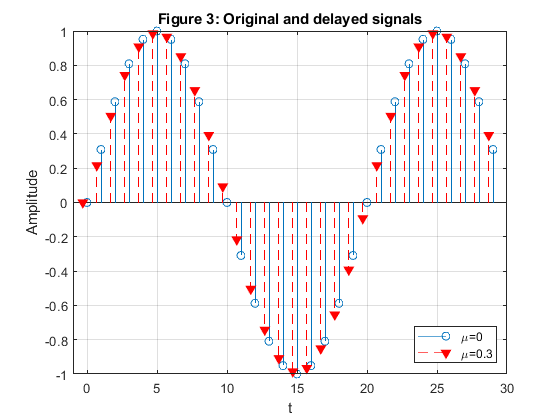
Generate the first 30 samples of the signal x[n] = sin(0.1*pi*n)
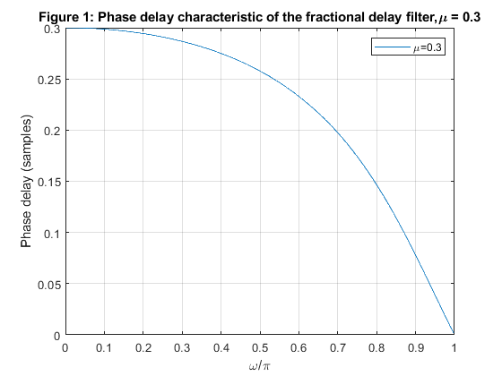
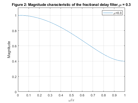
and perform the fractional delay filtering for the delay factor μ =
0.3.
Plot the input sequence {x[n]} and the delayed sequence {y[n]}.
Used functions: freqz, phasedelay (Signal Processing Toolbox), dfilt.farrowlinearfd (DSP System Toolbox)
clear all, close all
mu = 0.3;
h = dfilt.farrowlinearfd(mu);                           % Design object for Farrow fractional delay filtering
[phi,f] = phasedelay(h,512,2);                          % Computing the phase delay
figure (1)
plot(f,phi/pi)
xlabel('\omega/\pi'), ylabel('Phase delay (samples)'), grid
title('Figure 1: Phase delay characteristic of the fractional delay filter,\mu = 0.3')
legend('\mu=0.3','Location','northeast');
[H,f] = freqz(h,512,2);                                 % Computing the frequency response
figure (2)
plot(f,abs(H))
xlabel('\omega/\pi'), ylabel('Magnitude'), axis([0,1,0,1.1]),grid
title('Figure 2: Magnitude characteristic of the fractional delay filter,\mu = 0.3')
legend('\mu=0.3','Location','northeast');
% Aplying the fractional delay filter
t = 0:29;
x = sin(pi*0.1*t);                                       % Original signal
y = filter(h,x);                                         % Delayed signal
figure (3)
stem(t,x); hold on; stem(t-0.3,y,'v--r','filled')
xlabel('t'),ylabel('Amplitude')
title('Figure 3: Original and delayed signals')
legend('\mu=0','\mu=0.3','Location','southeast'), grid
axis([-1,30,-1,1]);