Multirate Filtering for Digital Signal Processing: MATLAB® Applications, Chapter V: IIR Filters for Sampling Rate Conversion - Exercises
Contents
Exercise 5.1
Design and implementation of an IIR polyphase
interpolator.
a) Construct the factor-of-5 interpolator by making use of the efficient polyphase configuration
of Figure 5.7.
b) Use the polyphase all-pass branches given in Example 5.2.
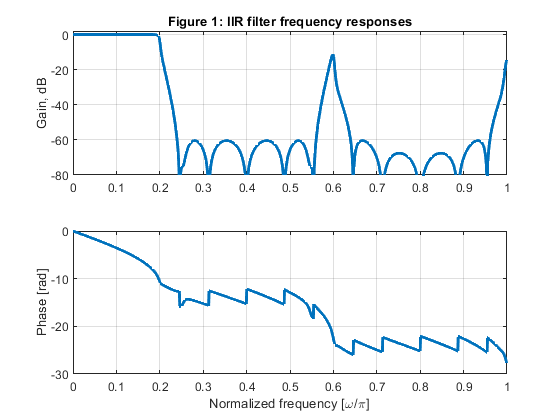
c) Compute and plot the magnitude and phase
responses of the interpolation filter.
d) Generate an input signal of the sampling frequency of 5000 Hz, and perform the factor-of-5
interpolation with the efficient IIR interpolator of Figure 5.7.
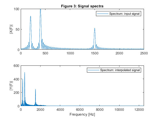
e) Plot the input and output spectra of the
signal.
f) Compute the multiplication rate of the system.
a) Commutative polyphase structure of the factor-of-L IIR interpolator (Figure 5.7 of the
book).
Used functions: freqz, upsample (Signal Processing Toolbox)
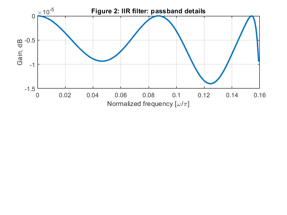
clear all, close all
% (b) Polyphase all-pass branches
% IIR filter poles from Example 5.2 of the book>
z01 = -0.03247627480; z02 = -0.4519480048; z03 = -0.9477051753;
z11 = -0.08029157130; z12 = -0.5548998293;
z21 = -0.1417079348;  z22 = -0.6883346404;
z31 = -0.2320513100;  z32 = -0.7961481351;
z41 = -0.3532045984;  z42 = -0.8755417392;
% Polyphase branches
a0 = conv([1,-z01],[1,-z02]); a0 = conv(a0,[1,-z03]);
a1 = conv([1,-z11],[1,-z12]);
a2 = conv([1,-z21],[1,-z22]);
a3 = conv([1,-z31],[1,-z32]);
a4 = conv([1,-z41],[1,-z42]);

A0=upsample(a0,5); A1=upsample(a1,5); A2=upsample(a2,5); A3=upsample(a3,5); A4=upsample(a4,5);
B0=fliplr(A0); B1=[0,fliplr(A1)]; B2=[0,0,fliplr(A2)]; B3=[0,0,0,fliplr(A3)]; B4=[0,0,0,0,fliplr(A4)];

% Computing the phase responses of polyphase branches
[PH0,f] = freqz(B0,A0,1024,2); [PH1,f] = freqz(B1,A1,1024,2); [PH2,f] = freqz(B2,A2,1024,2);
[PH3,f] = freqz(B3,A3,1024,2); [PH4,f] = freqz(B4,A4,1024,2);

% (c)   Frequency responses of the polyphase filter
H=PH0+PH1+PH2+PH3+PH4;
figure(1)
subplot(2,1,1), plot(f,20*log10(abs(H)/5),'LineWidth',2), grid
title('Figure 1: IIR filter frequency responses')
ylabel('Gain, dB'), axis([0,1,-80,2])
subplot(2,1,2), plot(f,unwrap(angle(H)),'LineWidth',2),grid
xlabel('Normalized frequency [\omega/\pi]'), ylabel('Phase [rad]')

% Plot the passband details:
figure (2)
subplot(2,1,1)
plot(f(1:164),20*log10(abs(H(1:164))/5),'LineWidth',2), grid
xlabel('Normalized frequency [\omega/\pi]'), ylabel('Gain, dB')
title('Figure 2: IIR filter: passband details')

% (d)   Generating the input signal {x[n]}
n = 0:200;
Fx = 5000;                                           % Sampling frequency at the input
x = 0.8*cos(2*pi*200*n/Fx) + cos(2*pi*400*n/Fx) + 0.5*cos(2*pi*1500*n/Fx);
[X,F1] = freqz(x,1,2000,5000);

% IIR filter, structure verification: polyphase filtering and upsampling
u0 = filter(fliplr(a0),a0,x); u1 = filter(fliplr(a1),a1,x); u2 = filter(fliplr(a2),a2,x);
u3 = filter(fliplr(a3),a3,x); u4 = filter(fliplr(a4),a4,x);
U = [u0;u1;u2;u3;u4];
y = U(:);                                             % Interpolated signal
[Y,F2] = freqz(y,1,2000,25000);

% e) Plot the input and output spectra of the interpolator
figure (3)
subplot(2,1,1), plot(F1,abs(X)), legend('Spectrum: input signal'), ylabel('|X(F)|'), axis([0,2500,0,100])
title('Figure 3: Signal spectra')
subplot(2,1,2),
plot(F2,abs(Y)), legend('Spectrum: interpolated signal'), ylabel('|Y(F)|'), xlabel('Frequency [Hz]')
axis([0,12500,0,600])

% (f)  Computing the multiplication rate
% Number of multipliers in all polyphase branches is
N = 11;
% Multiplication rate (the number of multiplications per second) R_M_INT is computed as:
R_M_INT = N*Fx;
disp('Multiplication rate of the factor-of-5 interpolator')
disp('Sampling rate conversion: 5000 Hz to 25000 Hz')
disp(['Number of multiplications per second: ', num2str(R_M_INT)]);
Multiplication rate of the factor-of-5 interpolator
Sampling rate conversion: 5000 Hz to 25000 Hz
Number of multiplications per second: 55000
Exercise 5.2
For the factor-of-5 interpolator designed in the MATLAB Exercise 5.1,
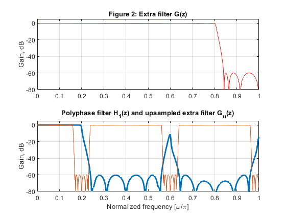
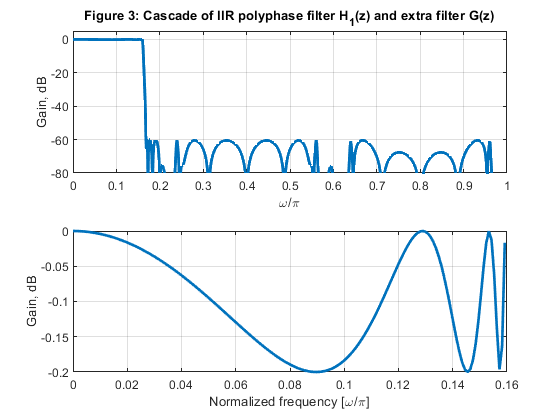
design an IIR extra filter to provide the overall system satisfying Case
a tolerance scheme.
Compute the multiplication rate of the system consisting of the extra filter and factor-of-5 interpolator.
Filter specification: Case a tolerance scheme (from Figure 3.5 of
the book).
Interpolator with the extra filter G(z) at the input
(Figure 5.12(b) of the book).
Used functions: ellip, freqz, upsample (Signal Processing Toolbox)
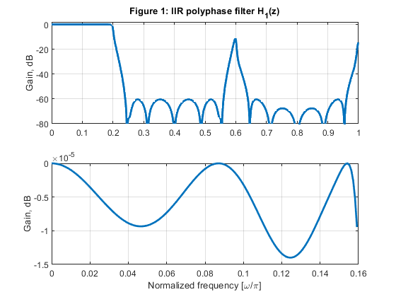
clear all, close all
% The design procedure is performed in three steps:
%    STEP 1: Design of IIR polyphase filter H1(z) as given in Exercise 5.1 to satisfy Case c tolerance scheeme.
%    STEP 2: Design the extra filter G(z) to achieve Case a tolerance
%    scheme.
%    STEP 3: Compute the multiplication rate.

% STEP 1: Design of IIR polyphase filter H1(z) as given in Exercise 5.1:
% IIR filter poles
z01 = -0.03247627480; z02 = -0.4519480048; z03 = -0.9477051753;
z11 = -0.08029157130; z12 = -0.5548998293;
z21 = -0.1417079348;  z22 = -0.6883346404;
z31 = -0.2320513100;  z32 = -0.7961481351;
z41 = -0.3532045984;  z42 = -0.8755417392;
% Polyphase branches
a0 = conv([1,-z01],[1,-z02]); a0 = conv(a0,[1,-z03]);
a1 = conv([1,-z11],[1,-z12]);
a2 = conv([1,-z21],[1,-z22]);
a3 = conv([1,-z31],[1,-z32]);
a4 = conv([1,-z41],[1,-z42]);

A0=upsample(a0,5); A1=upsample(a1,5); A2=upsample(a2,5); A3=upsample(a3,5); A4=upsample(a4,5);
B0=fliplr(A0); B1=[0,fliplr(A1)]; B2=[0,0,fliplr(A2)]; B3=[0,0,0,fliplr(A3)]; B4=[0,0,0,0,fliplr(A4)];
% Computing the phase responses of polyphase branches
[PH0,f] = freqz(B0,A0,1024,2); [PH1,f] = freqz(B1,A1,1024,2); [PH2,f] = freqz(B2,A2,1024,2);
[PH3,f] = freqz(B3,A3,1024,2); [PH4,f] = freqz(B4,A4,1024,2);
% The polyphase IIR filter frequency response
H1=PH0+PH1+PH2+PH3+PH4;
figure(1)
subplot(2,1,1), plot(f,20*log10(abs(H1)/5),'LineWidth',2), grid
ylabel('Gain, dB'), axis([0,1,-80,2])
title('Figure 1: IIR polyphase filter H_1(z)')
% Plot the passband details:
figure (1)
subplot(2,1,2)
plot(f(1:164),20*log10(abs(H1(1:164))/5),'LineWidth',2), grid
xlabel('Normalized frequency [\omega/\pi]'), ylabel('Gain, dB')

% STEP 2: Extra filter
[b,a]=ellip(7,0.2,60,0.80);                % Elliptic extra filter design
[G,f]=freqz(b,a,1024,2);                   % Extra filter frequency response
bb=upsample(b,5);                          % Extra filter: upsampling-by-5
aa=upsample(a,5);                          % Extra filter: upsampling-by-5
[Gu,f]=freqz(bb,aa,1024,2);                % Frequency response of upsampled-by-5 extra filter
figure (2)
subplot(2,1,1)
plot(f,20*log10(abs(G)),'r')
ylabel('Gain, dB'), axis([0,1,-80,5])
title('Figure 2: Extra filter G(z)')
grid
subplot(2,1,2)
plot(f,20*log10(abs(H1)/5),'LineWidth',2), grid
hold on
plot(f,20*log10(abs(Gu)))
axis([0,1,-80,5])
xlabel('Normalized frequency [\omega/\pi]'), ylabel('Gain, dB')
title('Polyphase filter H_1(z) and upsampled extra filter G_u(z)')

Hover=(H1/5).*Gu;                          % Overall filter: frequency response of the single-stage equivalent
figure (3)
subplot(2,1,1)
plot(f,20*log10(abs(Hover)),'LineWidth',2)
xlabel('\omega/\pi'), ylabel('Gain, dB'), axis([0,1,-80,5])
title('Figure 3: Cascade of IIR polyphase filter H_1(z) and extra filter G(z)')
grid
% Plot the passband details:
figure (3)
subplot(2,1,2)
plot(f(1:164),20*log10(abs(Hover(1:164))),'LineWidth',2), grid
xlabel('Normalized frequency [\omega/\pi]'), ylabel('Gain, dB')

% STEP 3: Computing the multiplication rate (the number of multiplications per second) R_M_INT
Fx = 5000;                                 % The input sampling frequency of the interpolator of Exercise 5.1
% Multiplication rate of the interpolation polyphase filter:
Np = 11; % Number of multiplication constants in polyphase filter
R_M_INT = Np*Fx;
% Multiplication rate of the extra filter:
Ne = 7; % Number of multiplication constants in extra filter
R_M_EX = Ne*Fx;
% Multiplication rate of the system R_M_S
R_M_S = R_M_INT + R_M_EX;
disp('Multiplication rate of the factor-of-5 interpolator composed of extra filter and polyphase interpolator')
disp('Sampling rate conversion: 5000 Hz to 25000 Hz')
disp(['Number of multiplications per second: ', num2str(R_M_S)]);
Multiplication rate of the factor-of-5 interpolator composed of extra filter and polyphase interpolator
Sampling rate conversion: 5000 Hz to 25000 Hz
Number of multiplications per second: 90000
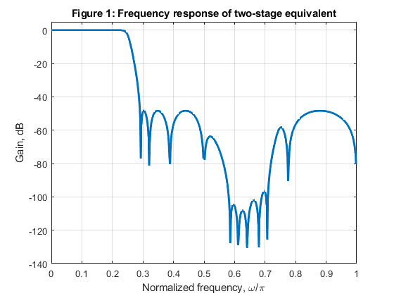
Exercise 5.3
Two-stage decimation with M = 4.
a) Design the 7th order halfband filter with the stopband edge frequency
ωs = 0.58π. (Use the program halfbandiir.)
b) Construct the two-stage decimator using the efficient configuration
of Figure 5.15(a).
c) Compute and plot the magnitude response of the single-stage
equivalent.
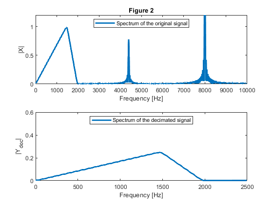
d) Generate an input signal of the sampling frequency 20000 Hz, and decimate this signal by 4 using the two-stage decimator designed above.
e) Compute and plot the input and output spectra of the signal.
f) Compute the multiplication rate of the system.
Efficient commutative structure for factor-of-two decimator.
(Figure 5.15(a) of the book).
Used functions: fir2, freqz, upsample (Signal Processing Toolbox), halfbandiir, (Appendix)
close all, clear all

% (a)   7th order IIR half-band filter
Nord = 7;                                                 % Filter order
Fs = 0.58;                                                % Stopband edge frequency
Fp = 1-Fs;                                                % Passband edge frequency
[b,a,z,p,k] = halfbandiir(Nord,Fp);                       % Halfband IIR filter design

% (b)  Two stage decimator: computation of the coefficients in all-pass branches
% A0(z) and A1(z):
pp = sort(abs(p));
beta0 = (abs(pp(2)))^2;    beta1 = (abs(pp(4)))^2;  beta2 = (abs(pp(6)))^2;
A0_a = conv([beta0,1],[beta2,1]); A0_b = fliplr(A0_a);
A1_a = [beta1,1]; A1_b = fliplr(A1_a);

% (c)   Frequency response of the single stage equivalent
[H0,f] = freqz(b,a,512,2);
[H1,f] = freqz(upsample(b,2),upsample(a,2),512,2);
H = H0.*H1;
figure (1)
plot(f,20*log10(abs(H)),'LineWidth',2),axis([0,1,-140,5]), grid
xlabel('Normalized frequency, \omega/\pi'),ylabel('Gain, dB')
title ('Figure 1: Frequency response of two-stage equivalent')

% (d)     Generating the input signal
Fx = 20000;                                             % Sampling frequency of the original signal
F = [0,3000/Fx,4000/Fx,1]; A=[0,1,0,0]; x1 = fir2(512,F,A);
x = x1 + 0.003*cos(2*pi*4400*(0:512)/Fx) + 0.008*cos(2*pi*8000*(0:512)/Fx);% Original signal

% Decimation-by-4:

% 1st stage: decimation-by-2
u0 = x(1:2:length(x));
u1 = [0,x(2:2:length(x)-1)];
y0 = filter(A0_a,A0_b,u0);
y1 = filter(A1_a,A1_b,u1);
yst = (y0 + y1)/2;                                        % Original signal decimated by 2

% 2nd stage: decimation-by-2
u0 = yst(1:2:length(yst));
u1 = [0,yst(2:2:length(yst)-1)];
y0 = filter(A0_a,A0_b,u0);
y1 = filter(A1_a,A1_b,u1);
ydec = (y0 + y1)/2;                                       % Original signal decimated by 4

%(e)    Compute and plot the input and output spectra of the signal
[X,f] = freqz(x,1,1000,20000); % Spectrum of the original signal
figure (2)
subplot(2,1,1)
plot(f,abs(X),'LineWidth',2)
xlabel('Frequency [Hz]'), ylabel('|X|'), axis([0,Fx/2,0,1.2])
legend('Spectrum of the original signal','Location','north')
title ('Figure 2')
[Ydec,fd] = freqz(ydec,1,1000,Fx/4);
subplot(2,1,2)
plot(fd,abs(Ydec),'LineWidth',2), xlabel('Frequency [Hz]'),ylabel('|Y_{dec}|'), axis([0,Fx/8,0,0.6])
legend('Spectrum of the decimated signal','Location','north')

% (f)   Computation of the multiplication rate
% Number of multiplication constants per stage N:
N = 3;
% Multiplication rate of two stage decimator
R_M_DEC = N*Fx/2 + N*Fx/4;                                 % Multiplications per second
disp('Multiplication rate of two stage decimator')
disp('Sampling rate conversion: 20000 Hz to 2500 Hz')
disp(['Number of multiplications per second: ', num2str(R_M_DEC)]);
Multiplication rate of two stage decimator
Sampling rate conversion: 20000 Hz to 2500 Hz
Number of multiplications per second: 45000

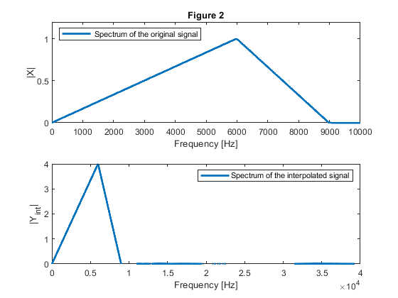
Exercise 5.4
Two-stage interpolator with L = 4.
a) Design the 7th order halfband filter with the stopband edge frequency
ωs = 0.58π. (Use the program halfbandiir.)
b) Construct the two-stage interpolator using the efficient configuration
of Figure 5.15(b).
c) Compute and plot the magnitude response of the single-stage
equivalent.
d) Generate an input signal of the sampling frequency 20000 Hz, and interpolate this signal by 4 using the two-stage interpolator designed above.
e) Compute and plot the input and output spectra of the signal.
f) Compute the multiplication rate of the system.
Efficient commutative structure for factor-of-two interpolator.
(Figure 5.15(b) of the book).
Used functions: fir2, freqz, % upsample (Signal Processing Toolbox), halfbandiir, (Appendix)
 close all, clear all

% (a)   7th order IIR half-band filter
Nord = 7;                                                 % Filter order
Fs = 0.58;                                                % Stopband edge frequency
Fp = 1-Fs;                                                % Passband edge frequency
[b,a,z,p,k] = halfbandiir(Nord,Fp);                       % Halfband IIR filter design

% (b)  Two stage interpolator: computation of the coefficients in all-pass branches
% A0(z) and A1(z):
pp = sort(abs(p));
beta0 = (abs(pp(2)))^2;    beta1 = (abs(pp(4)))^2;  beta2 = (abs(pp(6)))^2;
A0_a = conv([beta0,1],[beta2,1]); A0_b = fliplr(A0_a);
A1_a = [beta1,1]; A1_b = fliplr(A1_a);

% (c)    Frequency response of the single stage equivalent
[H0,f] = freqz(upsample(b,2),upsample(a,2),512,2);
[H1,f] = freqz(b,a,512,2);
H = H0.*H1;
figure (1)
plot(f,20*log10(abs(H)),'LineWidth',2),axis([0,1,-140,5]),grid
xlabel('Normalized frequency, \omega/\pi'),ylabel('Gain, dB')
title ('Figure 1: Frequency response of two-stage equivalent')

% (d)     Generating the input signal
Fx = 20000;                                               % Sampling frequency of the original signal
F = [0,2*6000/Fx,2*9000/Fx,1]; A=[0,1,0,0]; x = fir2(512,F,A); % Original signal

% Interpolation-by-4:

% 1st stage: interpolation-by-2
y0 = filter(A0_a,A0_b,x);
y1 = filter(A1_a,A1_b,x);
yy = [y0;y1];
yst = yy(:);                                              % Original signal interpolated by 2

% 2nd stage: interpolation-by-2
y00 = filter(A0_a,A0_b,yst');
y11 = filter(A1_a,A1_b,yst');
yy2 = [y00;y11];
yint = yy2(:);                                            % Original signal interpolated by 4

%(e) Compute and plot the input and output spectra of the signal
[X,f] = freqz(x,1,1000,Fx); % Spectrum of the original signal
figure (2)
subplot(2,1,1)
plot(f,abs(X),'LineWidth',2)
legend(' Spectrum of the original signal','Location','northwest')
xlabel('Frequency [Hz]'), ylabel('|X|'), axis([0,Fx/2,0,1.2])
title ('Figure 2')
[Yint,fi] = freqz(yint,1,8000,Fx*4);
subplot(2,1,2)
plot(fi,abs(Yint),'LineWidth',2), xlabel('Frequency [Hz]'),ylabel('|Y_{int}|')
legend('Spectrum of the interpolated signal','Location','northeast')

% (f) Computation of the multiplication rate
% Number of multiplication constants per stage N:
N = 3;
% Multiplication rate of two stage interpolator
R_M_INT = N*Fx + N*Fx*2;                                  % Multiplications per second
disp('Multiplication rate of two stage interpolator')
disp('Sampling rate conversion 20000 Hz to 80000 Hz')
disp(['Number of multiplications per second: ', num2str(R_M_INT)]);
Multiplication rate of two stage interpolator
Sampling rate conversion 20000 Hz to 80000 Hz
Number of multiplications per second: 180000
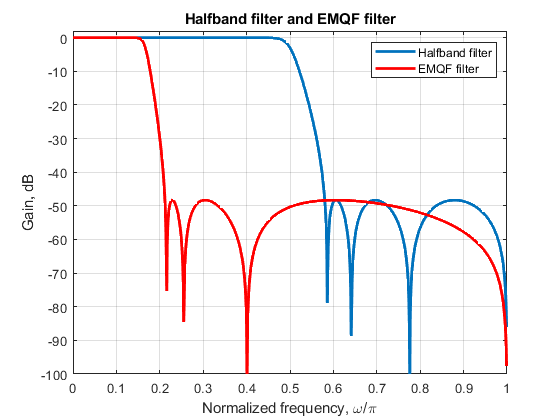
Exercise 5.5
Design the 7th order EMQF filter with 3 dB cut-off frequency ω3dB = (1/6)π
starting from the 7th order halfband filter from MATLAB Exercise 5.3. (Use the program halfbandiir.)
Use the transformation formulae (5.43) - (5.45) from the book.
Compute the passband and stopband edge frequencies of the resulting EMQF filter.
Compute and plot the magnitude responses
of the start-up halfband filter and the magnitude response of the EMQF filter.
Used functions: freqz, (Signal Processing Toolbox), halfbandiir, (Appendix)
 close all, clear all
%  The passband edge frequency of the halfband filter Fp:
Fs_HB = 0.58;                                              % See specifications for Example 5.3: omega_s = 0.58*pi
Fp_HB = 1-Fs_HB;                                           % Calculated from the stopband edge frequency Fs.
%
%  7th order IIR half-band filter
N = 7;
[b,a,z,p,k] = halfbandiir(N,Fp_HB);                        % Halfband filter design

pp = sort(abs(p).^2);

% Computing the coefficients of halfband filter all-pass branches
alpha = 0;
alpha1 = 0;
beta_HB = pp(2:2:length(pp));
p1 = [1 alpha1];
for ind = 2:2:(N-1)/2
  p1 = conv(p1,[1 alpha*(1+beta_HB(ind)) beta_HB(ind)]);
end
p2 = 1;
for ind = 1:2:(N-1)/2
  p2 = conv(p2,[1 alpha*(1+beta_HB(ind)) beta_HB(ind)]);
end

% Halfband filter all-pass branches
A1HBd = p1;
A1HBn = fliplr(A1HBd);
A0HBd = p2;
A0HBn = fliplr(A0HBd);

% Frequency responses of halfband filter all-pass branches
[A0,f] = freqz(A0HBn,A0HBd,1000,2);
[A1,f] = freqz(A1HBn,A1HBd,1000,2);

H_HB   = (A0+A1)/2;                                        % Frequency response of halfband filter
figure (1)
plot(f,20*log10(abs(H_HB)),'LineWidth',2)
hold on

% EMQF filter
F3dB=1/6; % 3-dB cutoff frequency

% Frequency transformations according the transformation formulae (5.43)-(5.45):
alpha = -cos(pi*F3dB);                                     % Formula (5.43)
alpha1 = (1-sqrt(1-alpha^2))/alpha;                        % Formula (5.44)
beta = (beta_HB+alpha1^2)./(beta_HB*alpha1^2+1);           % Formula (5.45)

% Computing the coefficients of EMQF filter all-pass branches
p1 = [1 alpha1];
for ind = 2:2:(N-1)/2
  p1 = conv(p1,[1 alpha*(1+beta(ind)) beta(ind)]);
end
p2 = 1;
for ind = 1:2:(N-1)/2
  p2 = conv(p2,[1 alpha*(1+beta(ind)) beta(ind)]);
end

% EMQF filter all-pass branches
A1d = p1;
A1n = fliplr(A1d);
A0d = p2;
A0n = fliplr(A0d);

% Frequency responses of EMQF filter all-pass branches
[A0,f] = freqz(A0n,A0d,1000,2);
[A1,f] = freqz(A1n,A1d,1000,2);

H_EMQF   = (A0+A1)/2;                                      % Frequency response of EMQF filter
figure (1)
plot(f,20*log10(abs(H_EMQF)),'r','LineWidth',2), grid, axis([0,1,-100,2])
xlabel('Normalized frequency, \omega/\pi'), ylabel('Gain, dB')
title('Halfband filter and EMQF filter')
legend('Halfband filter', 'EMQF filter','Location','northeast')

% Computing the edge frequencies of EMQF filter
ksi = tan(Fs_HB*pi/2)/tan(Fp_HB*pi/2);                      % Selectivity factor
Fp = 2*atan(tan(F3dB*pi/2)/sqrt(ksi))/pi;                   % Passband edge frequency
Fs = 2*atan(tan(F3dB*pi/2)*sqrt(ksi))/pi;                   % Stopband edge frequency
disp('Edge frequencies of EMQF filter')
disp(['Passband edge frequency Fp: ', num2str(Fp)]);
disp(['Stopband edge frequency Fs: ', num2str(Fs)]);
Edge frequencies of EMQF filter
Passband edge frequency Fp: 0.13046
Stopband edge frequency Fs: 0.21174
Exercise 5.6
Compute the multiplication rate of the three-stage decimator of Example 5.6 (pages 165-167 in the book) for the input sampling frequency of 2000 Hz.
close all, clear all
%   In this Exercise, we examine the multiplication rate of the factor-of-30 IIR decimator
%   implemented in three-stages with M_1 = 5, M_2 = 3, M_3 = 2.
%   The input sampling frequency Fx:

Fx = 2000;                                                  % Sampling frequency at the input

% Number of multipliers per stage as given in Table 5.2
Nmult1 = 3;                                                 % Number of multipliers in the first-stage decimation filter
Nmult2 = 4;                                                 % Number of multipliers in the second-stage decimation filter
Nmult3 = 4;                                                 % Number of multipliers in the third-stage decimation filter

% The multiplication rate of three-stage factor-of-30 decimator with
% M_1 = 5, M_2 = 3, M_3 = 2:
R_M_DEC = Nmult1*Fx + Nmult2*Fx/5 + Nmult3*Fx/(5*3*2);      % Number of multiplications per second in the three stage decimator
disp(['Number of multiplications per second in the three stage decimator: ', num2str(R_M_DEC)]);
% Comments:
% 1. In the first-stage decimation filter, arithmetic operations are
% evaluated at the input sampling rate Fx = 2000 Hz
% 2. In the second-stage decimation filter, arithmetic opearations are
% evaluated at the sampling rate Fx/5 = 2000/5 Hz
% 3. In the third-stage decimation filter, which is a halfband filter,
% the arithmetic operations can be evaluated at the sampling rate Fx/(5x3x2)=
% 2000/(5x3x2) Hz
Number of multiplications per second in the three stage decimator: 7866.6667
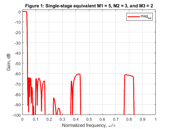
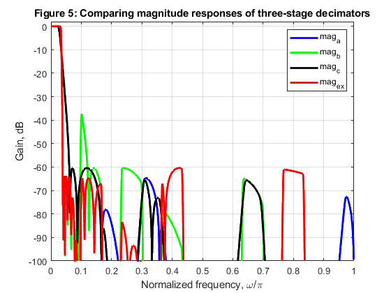
Exercise 5.7
The factor-of-30 decimator of Example 5.6 is implemented in three stages where M1 = 5,
M2 = 3, and M3 = 2.
The parameters of the EMQF filters are given in Table 5.2. (Use the program emqf_des.)
Examine the frequency response of the single-stage equivalents for the
following combinations:
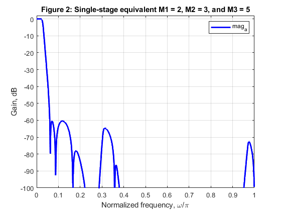
a) M1 = 2, M2 = 3, and M3 = 5
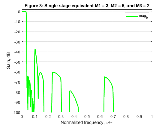
b) M1 = 3, M2 = 5, and M3 = 2
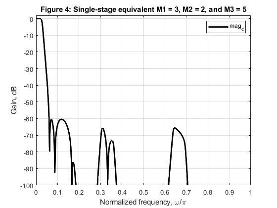
c) M1 = 3, M2 = 2, and M3 = 5
Compute and plot the magnitude characteristics of the single-stage equivalents defined above,
and compare with the characteristic of Figure 5.23 (page 166 in the book).
Used functions: freqz, upsample (Signal Processing Toolbox), emqf_des, (Appendix)
close all, clear all
% Firstly, let us repeat the design procedure  of decimation filters of example 5.6: H_1(z), H_2(z), and H_3(z)
% using the design parameters given in Table 5.2 (page 167 in the book).

% H_1(z) is to be designed for the factor-of-5 decimator.
% H_1(z) is an EMQF filter with the following parameters:
N = 5;                                                % Filter order
alpha = -(1-1/8-1/64);                                % Common constant for the second-order sections
Fp = 0.0658;                                          % Passband edge frequency
F3dB = 0.1502;                                        % 3-dB cutoff frequency
Fs = 0.3240;                                          % Stopband edge frequency
[A0dH1,A0nH1,A1dH1,A1nH1] = emqf_des(N,alpha,Fp,Fs);  % EMQF filter design

% H_2(z) is to be designed for the factor-of-3 decimator.
% H_2(z) is an EMQF filter with the following parameters:
N = 7;                                                % Filter order
alpha = -1/2;                                         % Common constant for the second-order sections
Fp = 0.2172;                                          % Passband edge frequency
F3dB = 0.3334;                                        % 3-dB cutoff frequency
Fs = 0.4800;                                          % Stopband edge frequency
[A0dH2,A0nH2,A1dH2,A1nH2] = emqf_des(N,alpha,Fp,Fs);  % EMQF filter design

% H_3(z) is to be designed for the factor-of-2 decimator.
% H_3(z) is an EMQF filter with the following parameters:
N = 9;                                                 % Filter order
alpha = 0;                                             % Common constant for the second-order sections
Fp = 0.4200;                                           % Passband edge frequency
F3dB = 0.5000;                                         % 3-dB cutoff frequency
Fs = 0.5800;                                           % Stopband edge frequency
[A0dH3,A0nH3,A1dH3,A1nH3] = emqf_des(N,alpha,Fp,Fs);   % EMQF filter design

% EXEMINING THREE-STAGE FACTOR-OF-30 DECIMATORS: Frequency responses of single-stage equivalents:

% STEP 1: Let us generate single-stage equivalent of Example 5.6 (see pages 165-167 in the book):
% M1 = 5, M2 = 3, and M3 = 2
% The single stage equivalent: H_1(z)H_2(z^5)H_3(z^15)
[A0,f] = freqz(A0nH1,A0dH1,1000,2);
[A1,f] = freqz(A1nH1,A1dH1,1000,2);
H_1 = (A0+A1)/2;
[A0,f] = freqz(upsample(A0nH2,5),upsample(A0dH2,5),1000,2);
[A1,f] = freqz(upsample(A1nH2,5),upsample(A1dH2,5),1000,2);
H_2_5 = (A0+A1)/2;
[A0,f] = freqz(upsample(A0nH3,15),upsample(A0dH3,15),1000,2);
[A1,f] = freqz(upsample(A1nH3,15),upsample(A1dH3,15),1000,2);
H_3_15 = (A0+A1)/2;
mag_ex = (abs(H_1).*abs(H_2_5)).*abs(H_3_15);            % Magnitude response of the single-stage equivalent (5x3x2)
figure (1)
plot(f,20*log10(mag_ex),'r','LineWidth',2), grid, axis([0,1,-100,2])
xlabel('Normalized frequency, \omega/\pi'), ylabel('Gain, dB')
title('Figure 1: Single-stage equivalent M1 = 5, M2 = 3, and M3 = 2')
legend('mag_e_x')

% STEP 2: Generating single-stage equivalents for cases (a), (b), and (c) as requested:
% (a) M1 = 2, M2 = 3, and M3 = 5
% The single stage equivalent: H_3(z)H_2(z^2)H_1(z^6)
[A0,f] = freqz(A0nH3,A0dH3,1000,2);
[A1,f] = freqz(A1nH3,A1dH3,1000,2);
H_3 = (A0+A1)/2;
[A0,f] = freqz(upsample(A0nH2,2),upsample(A0dH2,2),1000,2);
[A1,f] = freqz(upsample(A1nH2,2),upsample(A1dH2,2),1000,2);
H_2_2 = (A0+A1)/2;
[A0,f] = freqz(upsample(A0nH1,6),upsample(A0dH1,6),1000,2);
[A1,f] = freqz(upsample(A1nH1,6),upsample(A1dH1,6),1000,2);
H_1_6 = (A0+A1)/2;
mag_a = (abs(H_3).*abs(H_2_2)).*abs(H_1_6);               % Magnitude response of the single-stage equivalent (2x3x5)
figure (2)
plot(f,20*log10(mag_a),'b','LineWidth',2), grid, axis([0,1,-100,2])
xlabel('Normalized frequency, \omega/\pi'), ylabel('Gain, dB')
title('Figure 2: Single-stage equivalent M1 = 2, M2 = 3, and M3 = 5')
legend('mag_a')

% (b) M1 = 3, M2 = 5, and M3 = 2
% The single stage equivalent: H_2(z)H_1(z^3)H_3(z^15)
[A0,f] = freqz(A0nH2,A0dH2,1000,2);
[A1,f] = freqz(A1nH2,A1dH2,1000,2);
H_2 = (A0+A1)/2;
[A0,f] = freqz(upsample(A0nH1,3),upsample(A0dH1,3),1000,2);
[A1,f] = freqz(upsample(A1nH1,3),upsample(A1dH1,3),1000,2);
H_1_3 = (A0+A1)/2;
[A0,f] = freqz(upsample(A0nH3,15),upsample(A0dH3,15),1000,2);
[A1,f] = freqz(upsample(A1nH3,15),upsample(A1dH3,15),1000,2);
H_3_15 = (A0+A1)/2;
mag_b = (abs(H_2).*abs(H_1_3)).*abs(H_3_15);               % Magnitude response of the single-stage equivalent (3x5x2)
figure (3)
plot(f,20*log10(mag_b),'g','LineWidth',2), grid, axis([0,1,-100,2])
xlabel('Normalized frequency, \omega/\pi'), ylabel('Gain, dB')
title('Figure 3: Single-stage equivalent M1 = 3, M2 = 5, and M3 = 2')
legend('mag_b')

% (c) M1 = 3, M2 = 2, and M3 = 5
% The single stage equivalent: H_3(z)H_2(z^2)H_1(z^6)
[A0,f] = freqz(A0nH2,A0dH2,1000,2);
[A1,f] = freqz(A1nH2,A1dH2,1000,2);
H_2 = (A0+A1)/2;
[A0,f] = freqz(upsample(A0nH3,3),upsample(A0dH3,3),1000,2);
[A1,f] = freqz(upsample(A1nH3,3),upsample(A1dH3,3),1000,2);
H_3_3 = (A0+A1)/2;
[A0,f] = freqz(upsample(A0nH1,6),upsample(A0dH1,6),1000,2);
[A1,f] = freqz(upsample(A1nH1,6),upsample(A1dH1,6),1000,2);
H_1_6 = (A0+A1)/2;
mag_c = (abs(H_2).*abs(H_3_3)).*abs(H_1_6);                % Magnitude response of the single-stage equivalent (3x2x5)
figure (4)
plot(f,20*log10(mag_c),'k','LineWidth',2), grid, axis([0,1,-100,2])
xlabel('Normalized frequency, \omega/\pi'), ylabel('Gain, dB')
title('Figure 4: Single-stage equivalent M1 = 3, M2 = 2, and M3 = 5')
legend('mag_c')

% Comparing magnitude responses:
figure (5)
plot(f,20*log10(mag_a),'b',f,20*log10(mag_b),'g',f,20*log10(mag_c),'k',f,20*log10(mag_ex),'r','LineWidth',2)
grid, axis([0,1,-100,2])
xlabel('Normalized frequency, \omega/\pi'), ylabel('Gain, dB')
title('Figure 5: Comparing magnitude responses of three-stage decimators')
legend('mag_a','mag_b','mag_c','mag_e_x')