Multirate Filtering for Digital Signal Processing: MATLAB® Applications, Chapter IV: FIR Filters for Sampling Rate Conversion - Exercises

Contents

Exercise 4.1

Study the polyphase decimation and interpolation by modifying program demo_4_1.
a)    Design an optimal linear-phase FIR filter to satisfy the Case b tolerance scheme of Figure 3.5 (b) for the sampling-rate conversion factor M = L = 4.
          The peak passband ripple is a_p = 0.1 dB, and the minimal stopband attenuation amounts to a_s = 60 dB.
          Choose the passband edge frequency ω_p < π/M.
          The sampling frequency at the input of decimator and at the output of interpolator is 12 kHz.
b)    Generate the input signal {x[n]} according to your own choice.
c)    Compute four polyphase components for the filter designed in point (a).
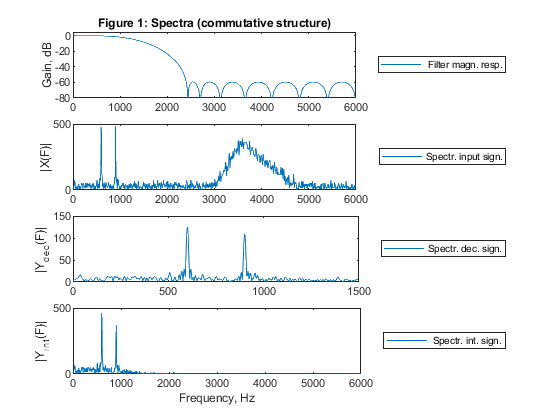
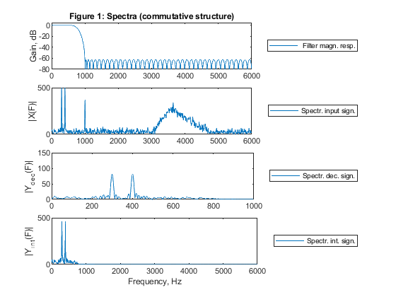
d)    Use the commutative polyphase structure of Figure 4.8 to decimate-by-4 signal {x[n]}. To perform decimation, modify Step 4 in program demo_4_1.
e)    Use the commutative polyphase configuration of Figure 4.10 to interpolate-by-4 decimated signal obtained in point (d). To perform interpolation, modify Step 5 in program demo_4_1.
f)    Compute the multiplication rate in decimator and in interpolator, respectively.
g)   Compute and plot: filter magnitude response, spectrum of the input signal, spectrum of the decimated signal, and spectrum of the interpolated signal.
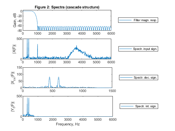
h)   Verify the commutative configurations used above:
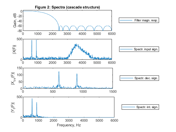
    (i) Evaluate decimation by using the cascade connection of FIR filter from point (a) and the factor-of-4 downsampler.
    (ii) Evaluate interpolation with the cascade of the factor-of-4 up-sampler and FIR filter from point (a).
    (iii) Compute and plot spectra of the decimated signal and that of the interpolated signal and compare with the results obtained in point (f).


Filter specification: Case b tolerance scheme (from Figure 3.5 of the book).


Commutative polyphase structure of a decimator (Figure 4.8 of the book).


Commutative polyphase structure of an interpolator (Figure 4.10 of the book).

Used functions:firpmord, firpm, fir2, freqz, downsample, upsample (Signal Processing Toolbox)

clear all, close all
% STEP 1-a),g)
% Lowpass FIR filter design
M = 4;                                    % Decimation factor
L = 4; % Interpolation factor
ap = 0.1; as = 60;                        % Specifying passband/stopband ripples
Fp = 0.1; Fs = 2/M-Fp;                    % Specifying passband/stopband boundary frequencies for Case b tolerance scheme
dev = [(10^(ap/20)-1)/(10^(ap/20)+1),  10^(-as/20)];  % Passband and stopband ripples
F = [Fp Fs];                              % Boundary frequencies
A = [1 0];                                % Desired amplitudes
[Nord,Fo,Ao,W]  = firpmord(F,A,dev);      % Estimating the filter order
Nord = Nord+2;                            % Increasing the Nord by 2 to provide some margin for Case b tolerance scheme
h = firpm(Nord,Fo,Ao,W);                  % Computing the filter coefficients
[H,F1] = freqz(h,1,1024,12000);           % Computation of filter frequency response
figure (1)
subplot(4,1,1), plot(F1,20*log10(abs(H))), title('Figure 1: Spectra (commutative structure)'), legend(' Filter magn. resp.','Location','eastoutside')
ylabel('Gain, dB'), axis([0,6000,-80,5])

% STEP 2-b),g)
Fx = 12000;
% Generating the input signal x
n = 0:1000;                               % Time index
ff = [0,0.1,0.5,0.6,0.8,1]; a = [0,0,0.05,0.9,0,0];
x = fir2(1000,ff,a);
x = 400*x+cos(2*pi*Fp/2*n)+cos(2*pi*3*Fp/4*n)+randn(size(n)); z=x;
[X,F1] = freqz(x,1,1024,12000);           % Computing the signal spectrum
subplot(4,1,2), plot(F1,abs(X)), legend('Spectr. input sign.','Location','eastoutside'), ylabel('|X(F)|'), axis([0,6000,0,500])
Fy=Fx/M;

% STEP 3-c)
% Polyphase decomposition
E = reshape(h,4,length(h)/4);

% STEP 4-d),g)
 % Polyphase downsampling and filtering
x0 = x(1:4:length(x)); x1 = [0,x(4:4:length(x))]; x2 = [0,x(3:4:length(x))];
x3 = [0,x(2:4:length(x))];
y0 = filter(E(1,:),1,x0); y1 = filter(E(2,:),1,x1); y2 = filter(E(3,:),1,x2); y3=filter(E(4,:),1,x3);
ydec = y0 + y1 + y2 + y3;                 % Decimated signal
[Ydec,F2] = freqz(ydec,1,512,3000);
subplot(4,1,3), plot(F2,abs(Ydec)), legend('Spectr. dec. sign.','Location','eastoutside'), ylabel('|Y_d_e_c(F)|'), axis([0,1500,0,150])

% STEP 5-e),g)
x = ydec;                                 % Input to the interpolator
% Poliphase filtering and up-sampling
u0 = L*filter(E(1,:),1,x); u1 = L*filter(E(2,:),1,x); u2 = L*filter(E(3,:),1,x);
u3 = L*filter(E(4,:),1,x);
U = [u0;u1;u2;u3];
yint = U(:);                              % Interpolated signal
[Yint,F3] = freqz(yint,1,1024,12000);
subplot(4,1,4), plot(F3,abs(Yint)); legend(' Spectr. int. sign.','Location','eastoutside'), xlabel('Frequency, Hz')
ylabel('|Y_i_n_t(F)|'), axis([0,6000,0,500])

% STEP 6-h)
 % Computing the multiplication rate in decimator and in interpolator
Rm_dec=(Nord+1)*Fx/M;
Rm_int=(Nord+1)*Fx/L;
disp('Multiplication rates of commutative structures')
disp(['Decimator (mult./second):    ', num2str(Rm_dec)]);
disp(['Interpolator (mult./second): ', num2str(Rm_int)]);
% STEP 7-h)
xf = filter(h,1,z);
xds = downsample(xf,M);
yus = upsample(xds,L);
yf = filter(L*h,1,yus);

figure (2)
subplot(4,1,1), plot(F1,20*log10(abs(H))), title('Figure 2: Spectra (cascade structure)'), legend(' Filter magn. resp.','Location','eastoutside'),
ylabel('Gain, dB'), axis([0,6000,-80,5])
subplot(4,1,2), plot(F1,abs(X)), legend('Spectr. input sign.','Location','eastoutside'), ylabel('|X(F)|'), axis([0,6000,0,500])
[Xds,Fds] = freqz(xds,1,512,3000);
subplot(4,1,3), plot(Fds,abs(Xds)), legend('Spectr. dec. sign.','Location','eastoutside'), ylabel('|X_d_s(F)|'), axis([0,1500,0,150])
[Yf,Fus] = freqz(yf,1,1024,12000);
subplot(4,1,4), plot(Fus,abs(Yf)); legend('Spectr. int. sign.','Location','eastoutside'), xlabel('Frequency, Hz')
ylabel('|Y_f(F)|'), axis([0,6000,0,500])

% Comparing Figures 1 and 2, we conclude that commutative structure consisting of 4 polyphase subfilters in parallel is successfully verified.
% Both figures display the identical results.

Multiplication rates of commutative structures
Decimator (mult./second):    60000
Interpolator (mult./second): 60000

Exercise 4.2

Simulate the process of polyphase decimation and interpolation by modifying program demo_4_2.
a)    Design an optimal linear-phase FIR filter to satisfy the Case a tolerance scheme of Figure 3.5 (a) for the sampling-rate conversion factor M = L = 6.
        The peak passband ripple is a_p = 0.1 dB, and the minimal stopband attenuation amounts to a_s = 60 dB.
        Choose the stopband edge frequency ω_s < π/M.
        The sampling frequency at the input of decimator and at the output of interpolator is 12 kHz.
b)    Generate the input signal {x[n]} according to your own choice.
c)    Compute six polyphase components for the filter designed in point (a).
d)    Simulate decimation-by-6 of the signal {x[n]} by making use of the commutative polyphase structure of Figure 4.8. To perform decimation, modify Step 4 in program demo_4_2.
e)    Simulate interpolation-by-6 of the decimated signal obtained in point (d) by making use of the commutative polyphase structure of Figure 4.10. To perform interpolation, modify Step 5 in program demo_4_2.
f)    Compute the multiplication rate in decimator and in interpolator, respectively.
g)    Compute and plot: filter magnitude response, spectrum of the input signal, spectrum of the decimated signal, and spectrum of the interpolated signal.
h)   Verify the commutative configurations used above:
   (i) Evaluate decimation by using the cascade connection of FIR filter from point (a) and the factor-of-6 downsampler.
   (ii) Evaluate interpolation with the cascade of the factor-of-6 up-sampler and FIR filter from point (a).
   (iii) Compute and plot spectra of the decimated signal and that of the interpolated signal and compare with the results obtained in point (f).


Filter specification: Case a tolerance scheme (from Figure 3.5 of the book).


Commutative polyphase structure of a decimator (Figure 4.8 of the book).


Commutative polyphase structure of an interpolator (Figure 4.10 of the book).

Used functions: firpmord, firpm, freqz, (Signal Processing Toolbox)

clear all, close all
% STEP 1-a),g)
% Lowpass FIR filter design
M = 6;                                     % Decimation factor
L = 6;                                     % Interpolation factor
ap = 0.1; as = 60;                         % Specifying passband/stopband ripples
Fp = 0.1; Fs = 1/M;                        % Specifying passband/stopband boundary frequencies for Case a tolerance scheme
dev = [(10^(ap/20)-1)/(10^(ap/20)+1),  10^(-as/20)];  % Passband and stopband ripples
F = [Fp Fs];                               % Boundary frequencies
A = [1 0];                                 % Desired amplitudes
[Nord,Fo,Ao,W]  = firpmord(F,A,dev); % Estimating the filter order
Nord = Nord+7;                             % Increasing the Nord by 7 to provide some margin for Case a tolerance scheme
h = firpm(Nord,Fo,Ao,W);                   % Computing the filter coefficients
[H,F1] = freqz(h,1,1024,12000);            % Computation of filter frequency response
figure (1)
subplot(4,1,1), plot(F1,20*log10(abs(H))), title('Figure 1: Spectra (commutative structure)'), legend(' Filter magn. resp.','Location','eastoutside')
ylabel('Gain, dB'), axis([0,6000,-80,5])

% STEP 2-b),g)
Fx = 12000;
% Generating the input signal
n = 0:1000; % Time index
ff = [0,0.1,0.5,0.6,0.8,1]; a = [0,0,0.05,0.9,0,0];
x = fir2(1000,ff,a);
x = 300*x+cos(2*pi*Fp/3*n)+cos(2*pi*Fp/4*n)+0.8*cos(pi*Fs*n)+randn(size(n)); z=x;
[X,F1] = freqz(x,1,1024,12000);           % Computing the signal spectrum
subplot(4,1,2), plot(F1,abs(X)), legend('Spectr. input sign.','Location','eastoutside'), ylabel('|X(F)|'), axis([0,6000,0,500])

% STEP 3-c)
 % Polyphase decomposition
 E = reshape(h,M,length(h)/M);

% STEP 4-d),g)
% Initial states in polyphase components
vk_i = zeros(size(E));
% Decimation
rot = 0;                                  % Initial rotator position
ydec = [];
for n=1:length(x)
    xn = x(n);
    vk = vk_i(rot+1,:); ek = E(rot+1,:);
    vk = [xn,vk(1:length(vk)-1)]; yn = sum(vk.*ek); % filtering
    vk_i(rot+1,:)=vk;
    if n==1, yy=0; end;
    if rot == 0, ss = 5; yy = yy+yn; ydec = [ydec,yy]; end;
    if rot == 1, ss = 0; yy = yy+yn; end;
    if rot == 2, ss = 1; yy = yy+yn; end;
    if rot == 3, ss = 2; yy = yy+yn; end;
    if rot == 4, ss = 3; yy = yy+yn; end;
    if rot == 5, ss = 4; yy = yn; end;
    rot = ss;
end
[Ydec,F2] = freqz(ydec,1,512,2000);
subplot(4,1,3), plot(F2,abs(Ydec)), legend('Spectr. dec. sign.','Location','eastoutside')
ylabel('|Y_d_e_c(F)|'), axis([0,1000,0,150])

% STEP 5-e),g)
% Interpolation
yi = 0; xk_i = zeros(size(E));
rot = 0;
k = 1;
for n=1:length(ydec)*L
    xn=ydec(k);
    xk = xk_i(rot+1,:); ek = E(rot+1,:);
    xk = [xn,xk(1:length(xk)-1)]; yn=sum(xk.*ek); % filtering
    xk_i(rot+1,:) = xk; yn=L*yn;
    if rot == 0 ss = 1; yi = [yi,yn]; end;
    if rot == 1 ss = 2; yi = [yi,yn]; end;
    if rot == 2 ss = 3; yi = [yi,yn]; end;
    if rot == 3 ss = 4; yi = [yi,yn]; end;
    if rot == 4 ss = 5; yi = [yi,yn]; end;
    if rot == 5 ss = 0; k = k+1; yi = [yi,yn]; end;
    rot = ss;
end
[Yint,F3] = freqz(yi,1,1024,12000);
subplot(4,1,4), plot(F3,abs(Yint)); legend('Spectr. int. sign.','Location','eastoutside')
xlabel('Frequency, Hz'), ylabel('|Y_i_n_t(F)|'), axis([0,6000,0,500])

% STEP 7-f)
% Computing the multiplication rate in decimator and in interpolator
Rm_dec = (Nord+1)*Fx/M;
Rm_int = (Nord+1)*Fx/L;
disp('Multiplication rates of commutative structures')
disp(['Decimator (mult./second):    ', num2str(Rm_dec)]);
disp(['Interpolator (mult./second): ', num2str(Rm_int)]);

% STEP 8-h)
xf = filter(h,1,z);
xds = downsample(xf,M);
yus = upsample(xds,L);
yf = filter(L*h,1,yus);

figure (2)
subplot(4,1,1), plot(F1,20*log10(abs(H))), title('Figure 2: Spectra (cascade structure)'),legend(' Filter magn. resp.','Location','eastoutside')
ylabel('Gain, dB'), axis([0,6000,-80,5]);
subplot(4,1,2), plot(F1,abs(X)), legend('Spectr. input sign.','Location','eastoutside'), ylabel('|X(F)|'), axis([0,6000,0,500])
[Xds,Fds] = freqz(xds,1,512,3000);
subplot(4,1,3), plot(Fds,abs(Xds)), legend('Spectr. dec. sign.','Location','eastoutside'), ylabel('|X_d_s(F)|'), axis([0,1500,0,150])
[Xus,Fus] = freqz(yf,1,1024,12000);
subplot(4,1,4), plot(Fus,abs(Xus)); legend(' Spectr. int. sign.','Location','eastoutside'), xlabel('Frequency, Hz'), ylabel('|Y_f(F)|'), axis([0,6000,0,500])

% Comments
% Exercise 4.2 is developed to simulate a sample-by-sample operation in the time-domain for a factor-of-6 decimator and for a factor-of-6 interpolator
% based on the efficient commutative polyphase structures.
% Comparing the figures 1 and 2 we conclude that commutative structure consisted of 6 polyphase subfilters in parallel is successfully verified.
% Both figures display the identical results.

Multiplication rates of commutative structures
Decimator (mult./second):    180000
Interpolator (mult./second): 180000

Exercise 4.3

Study the application of memory-saving structures of polyphase decimators and interpolators by modifying program demo_4_3.
a)    Design an optimal linear-phase FIR filter to satisfy the Case a tolerance scheme of Figure 3.5 (a), for the sampling-rate conversion factor M = L = 4.
      The peak passband ripple is a_p = 0.1 dB, and the minimal stopband attenuation is a_s = 50 dB.
      Choose the stopband edge frequency ω_s < π/M.
      The sampling frequency at the input of decimator and at the output of interpolator is 12 kHz.
b)    Generate the input signal {x[n]} according to your own choice.
c)    Compute four polyphase components for the filter designed in point (a).
d)    On the basis of the memory-saving structure of Figure 4.13 (from the book) develop the corresponding structure for M = 4. Decimate-by-4 signal {x[n]} by modifying Step 4 in the program demo_4_3.
e)    On the basis of the memory-saving structure of Figure 4.15 (from the book) develop the corresponding structure for L = 4. Interpolate-by-4 decimated signal by modifying Step 5 in the program demo_4_3.
f)    Compute the multiplication rate in decimator and in interpolator, respectively.
g)    Compute the number of delays in decimator and in interpolator, respectively.
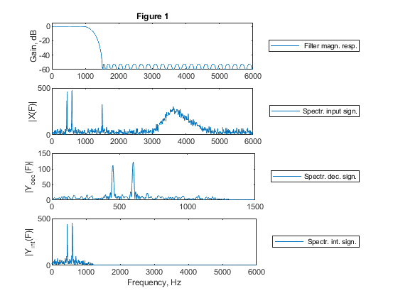
h)    Compute and plot: filter magnitude response, spectrum of the input signal, spectrum of the decimated signal, and spectrum of the interpolated signal.


Filter specification: Case a tolerance scheme (from Figure 3.5 of the book).

Used functions: firpm, fir2, freqz (Signal Processing Toolbox)

clear all, close all
% STEP 1:
% Lowpass FIR filter design
M = 4;                                             % Decimation factor
L = 4;                                             % Interpolation factor
Fx = 12000;
Fp = 0.15; Fs = 1/M; ap = 0.1; as = 50;            % Filter design parameters
h = firpm(55,[0,Fp,Fs,1],[1,1,0,0]);               % FIR filter design
[H,F1] = freqz(h,1,1024,12000);                    % Computing filter frequency response
figure (1)
subplot(4,1,1), plot(F1,20*log10(abs(H))), title('Figure 1')
legend(' Filter magn. resp.','Location','eastoutside'), ylabel('Gain, dB')
axis([0,6000,-60,5])

% STEP 2-b),g)
% Generating the input signal {x[n]}
n = 0:999;                                          % Time index
ff = [0,0.1,0.5,0.6,0.8,1]; a = [0,0,0.05,0.9,0,0];
x = fir2(999,ff,a);
x = 300*x+cos(2*pi*Fp/3*n)+cos(2*pi*Fp/4*n)+0.6*cos(pi*Fs*n)+randn(size(n)); z=x; % Input signal

[X,F1] = freqz(x,1,1024,12000);                     % Computing the signal spectrum
subplot(4,1,2), plot(F1,abs(X)), legend('Spectr. input sign.','Location','eastoutside'), ylabel('|X(F)|'), axis([0,6000,0,500])

% STEP 3:
% Polyphase decomposition
E = reshape(h,M,length(h)/M);
E = fliplr(E);

% STEP 4:
% Setting the initial states
xk = zeros(size(1:length(h)/M));
% Decimation
rot = 0; % Initial rotator position
ydec = [];
for n=1:length(x)
    xn = x(n); xk = xn*E((rot+1),:)+xk;
    if rot == 0 ss = 3; yn = xk(length(xk)); ydec = [yn,ydec]; xk = [0,xk(1:length(xk)-1)]; end;
    if rot == 1 ss = 0; end;
    if rot == 2 ss = 1; end;
    if rot == 3 ss = 2; end;
    rot = ss;
end;
[Ydec,F2] = freqz(ydec,1,512,3000);
subplot(4,1,3), plot(F2,abs(Ydec)), legend('Spectr. dec. sign.','Location','eastoutside'), ylabel('|Y_{dec}(F)|')
axis([0,1500,0,150])

% STEP 5:
% Interpolation
E = L*fliplr(E);
yi = [];
xk = zeros(size(1:length(h)/L));
rot = 0; % Initial rotator position
k = 1;
for n=1:length(ydec)*L
    xn = ydec(k); ek = E(rot+1,:);
    if k == 1,  xk = [xn,xk(1:length(xk)-1)]; end;
    yn = sum(xk.*ek); yi = [yi,yn];
    if rot == 0 ss = 1; end;
    if rot == 1 ss = 2; end;
    if rot == 2 ss = 3; end;
    if rot == 3 ss = 0; k = k+1; xk = [xn,xk(1:length(xk)-1)]; end;
    rot = ss;
end
[Yint,F3] = freqz(yi,1,1024,12000);
subplot(4,1,4)
plot(F3,abs(Yint));  legend(' Spectr. int. sign.','Location','eastoutside')
xlabel('Frequency, Hz'),ylabel('|Y_{int}(F)|')
axis([0,6000,0,500])

% STEP 6:
% Computation of the multiplication rate in decimator and in interpolator
Nf=length(h);                                       % FIR filter length
Rm_dec=Nf*Fx/M;                                     % Multiplication rate in decimator
Rm_int=Nf*Fx/L;                                     % Multiplication rate in interpolator
disp('Multiplication rates of decimator and interpolator')
disp(['Decimator (mult./second):    ', num2str(Rm_dec)]);
disp(['Interpolator (mult./second): ', num2str(Rm_int)]);

% STEP 7:
% Computation of the number of delays in decimator and in interpolator
Nd_dec=Nf/M;                                         % Number of delays in decimator
Nd_int=Nf/L;                                         % Number of delays in interpolator
disp('Number of delays in decimator and in interpolator')
disp(['Decimator:    ', num2str(Nd_dec)]);
disp(['Interpolator: ', num2str(Nd_int)]);
% Comments
% The number of delays in the memory-saving structure is determined according to the number of delays in the polyphase component of the highest order.
% Filter H(F) of the length N = 56 meets the design requirements specified in Exercise_4_3 and the factor-of-4 decimator and interpolator can be
% implemented with 4 polyphase subfilters where the length of each subfilter is 14, and they operate at the intermediate sampling rate of 3 kHz.

Multiplication rates of decimator and interpolator
Decimator (mult./second):    168000
Interpolator (mult./second): 168000
Number of delays in decimator and in interpolator
Decimator:    14
Interpolator: 14

Exercise 4.4

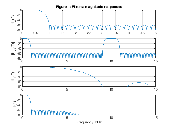
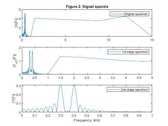
Investigate the efficiency of two-stage decimator by modifying program .demo_4_4 in such a manner that decimation-by-3 is followed by decimation-by-5.
Generate the corresponding plots to those given in Figures 4.19 and 4.20 (of the book).

Used functions: firpm, freqz, upsample (Signal Processing Toolbox)

close all, clear all
h1 = firpm(12,[0,0.5/15,9/15,12/15,1,1],[1,1,0,0,0,0],[1,5,5]); % Designing filter H1(z)
[H1,F1] = freqz(h1,1,1024,30);                                  % Frequency response  of H1(z)
h2 = firpm(59,[0,3*0.5/15,3*1/15,1],[1,1,0,0],[1,5]);           % Designing filter H2(z)
[H2,F2] = freqz(h2,1,1024,10);                                  % Frequency response of H2(z)
h2u = upsample(h2,3);                                           % Periodic filter H_2(z^3)
[H2u,F1] = freqz(h2u,1,1024,30);                                % Spectrum of the periodic filter H_2(z^3)
H = H1.*H2u;                                                    % The overall frequency response
figure (1)
subplot(4,1,1), plot(F2,20*log10(abs(H2))), ylabel('|H_2(F)|'), axis([0,5,-80,2]),grid
title('Figure 1: Filters: magnitude responses')
subplot(4,1,2), plot(F1,20*log10(abs(H2u))), ylabel('|H_2_u(F)|'),axis([0,15,-80,2]),grid
subplot(4,1,3), plot(F1,20*log10(abs(H1))), ylabel('|H_1(F)|'), axis([0,15,-80,2]),grid
subplot(4,1,4), plot(F1,20*log10(abs(H))), ylabel('|H(F)|'), axis([0,15,-80,2]),grid
xlabel('Frequency, kHz')

% Input signal
ff = [0,1/15,1.5/15,0.6,0.8,1]; a = [0,0,0.8,0.7,0.9,0];
x = fir2(990,ff,a);
x = 5*x+0.01*sin(2*pi*(1:991)*300/30000) + 0.01*sin(2*pi*(1:991)*400/30000);
[X,F1] = freqz(x,1,2048,30);                                    % Spectrum of the input signal
figure (2)
subplot(3,1,1), plot(F1,abs(X)), ylabel('|X(F)|'), legend('Original spectrum')
title('Figure 2: Signal spectra')

% Polyphase decomposition, M1 = 3
h1 = [h1,0,0];
E1 = reshape(h1,3,length(h1)/3);                                % Polyphase components
% Polyphase downsampling and filtering, M1 = 3
v0 = x(1:3:length(x)); v1 = [0,x(3:3:length(x))]; v2 = [0,x(2:3:length(x))];
y0 = filter(E1(1,:),1,v0); y1 = filter(E1(2,:),1,v1); y2 = filter(E1(3,:),1,v2);
yd1 = y0 + y1 + y2; % Decimated signal
[Yd1,F2]=freqz(yd1,1,2048,10);
subplot(3,1,2), plot(F2,abs(Yd1)), legend('1st stage spectrum'), ylabel('|Y_d_1(F)|')

% Polyphase decomposition, M2 = 5
E2 = reshape(h2,5,length(h2)/5);
% Polyphase downsampling and filtering, M2 = 5
x = yd1;
v0 = x(1:5:length(x)); v1 = [0,x(5:5:length(x))]; v2 = [0,x(4:5:length(x))];
v3 = [0,x(3:5:length(x))]; v4 = [0,x(2:5:length(x))];
y0 = filter(E2(1,:),1,v0); y1 = filter(E2(2,:),1,v1); y2 = filter(E2(3,:),1,v2);
y3 = filter(E2(4,:),1,v3); y4 = filter(E2(5,:),1,v4);
y = y0 + y1 + y2 + y3 + y4; % decimated signal
[Y,F3] = freqz(y,1,2048,2);
subplot(3,1,3), plot(F3,abs(Y)), legend('2nd stage spectrum'), ylabel('|Y(F)|')
xlabel('Frequency, kHz')

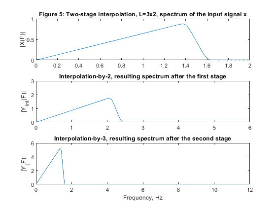
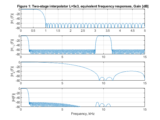
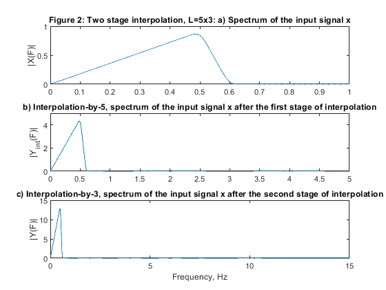
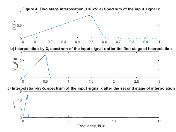
Exercise 4.5

Modify program demo_4_4 to study the two-stage implementation of factor-of-15 interpolator.
a)    Implement the interpolator with L₁ = 5 in the first stage, and L₂ = 3 in the second stage.
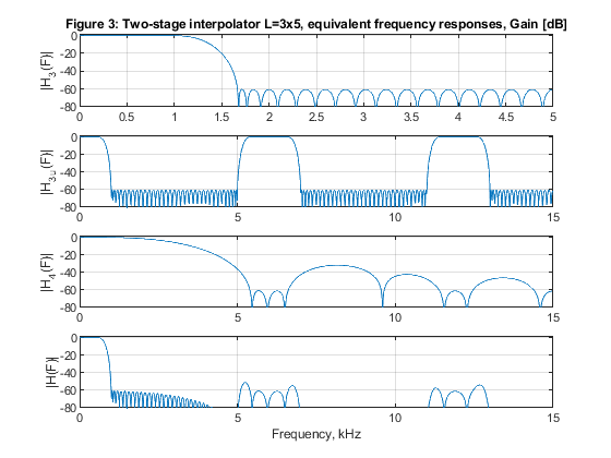
b)   Implement the interpolator with L₁ = 3 in the first stage, and L₂ = 5 in the second stage.
c)   Compare the computational efficiency of two solutions from (a) and (b).

Used functions: firpm, freqz, upsample (Signal Processing Toolbox)

close all, clear all
% STEP a): Design of two-stage factor-of-15 interpolator with L1=5 and L2=3.
L1=5; L2=3;
Fp=0.6; ap1=0.01/2; as=60; Fx=2000;                         % Design parameters for H1(z)
Nord_h1=73;                                                 % Selecting the filter order for H1(z)
h1 = firpm(Nord_h1,[0,0.6/5,1/5,1],[1,1,0,0],[1,3]);        % Filter H1(z)
[H1,F1] = freqz(h1,1,1024,10);                              % Frequency response  of H1(z)
Nord_h2=9;                                                  % Selecting the filter order for H2(z)
h2 = firpm(Nord_h2,[0,0.6/15,9.4/15,11.6/15,1,1],[1,1,0,0,0,0],[1,3,3]); % Filter H2(z)
[H2,F2] = freqz(h2,1,1024,30);                              % Frequency response of H2(z)
h1u = upsample(h1,3);                                       % Periodic filter H_2(z^5)
[H1u,F3] = freqz(h1u,1,1024,30); % Spectrum of the periodic filter H_2(z^3)
H = H1u.*H2;                                                % The overall frequency response
figure (1)
subplot(4,1,1), plot(F1,20*log10(abs(H1))), ylabel('|H_1(F)|'), axis([0,5,-80,2]),grid
title('Figure 1: Two-stage interpolator L=5x3, equivalent frequency responses, Gain [dB]');
subplot(4,1,2), plot(F3,20*log10(abs(H1u))), ylabel('|H_1_u(F)|'),axis([0,15,-80,2]),grid
subplot(4,1,3), plot(F2,20*log10(abs(H2))), ylabel('|H_2(F)|'), axis([0,15,-80,2]),grid
subplot(4,1,4), plot(F2,20*log10(abs(H))), ylabel('|H(F)|'), axis([0,15,-80,2]),grid
xlabel('Frequency, kHz')

% Input signal
ff = [0,0.5,0.6,1]; a = [0,0.9,0,0];
x = fir2(100,ff,a);
[X,F1] = freqz(x,1,2048,2);                                 % Spectrum of the input signal
figure (2)
subplot(3,1,1), plot(F1,abs(X)), ylabel('|X(F)|')
title('Figure 2: Two stage interpolation, L=5x3: a) Spectrum of the input signal x');

% Polyphase decomposition for the first stage with L1=5
h1=[h1,0];
E1 = reshape(h1,5,length(h1)/5);

% Input to the interpolator L1=5
% Poliphase filtering and up-sampling
u0 = L1*filter(E1(1,:),1,x); u1 = L1*filter(E1(2,:),1,x); u2 = L1*filter(E1(3,:),1,x);
u3 = L1*filter(E1(4,:),1,x); u4 = L1*filter(E1(5,:),1,x);
U = [u0;u1;u2;u3;u4];
yint = U(:);                                                % Interpolated signal
[Yint,F3] = freqz(yint,1,1024,10);
subplot(3,1,2), plot(F3,abs(Yint));  ylabel('|Y_i_n_t(F)|'), axis([0,5,0,5])
title('b) Interpolation-by-5, spectrum of the input signal x after the first stage of interpolation')

% Polyphase decomposition for the second stage with L2=3
z=yint';
h2=[h2,0,0];
E2=reshape(h2,3,length(h2)/3);

% Input to the interpolator L2=3
% Poliphase filtering and up-sampling
v0 = L2*filter(E2(1,:),1,z); v1 = L2*filter(E2(2,:),1,z); v2 = L2*filter(E2(3,:),1,z);
V = [v0;v1;v2];
y = V(:);                                                   % Interpolated signal
[Y,F3] = freqz(y,1,2048,30);
subplot(3,1,3), plot(F3,abs(Y)); ylabel('|Y(F)|'), axis([0,15,0,15])
title('c) Interpolation-by-3, spectrum of the input signal x after the second stage of interpolation'), xlabel('Frequency, Hz')

% STEP b): Design of two-stage factor-of-15 interpolator with L1=3 and L2=5.
L1=3; L2=5;
Nord_h3=44;
h3 = firpm(Nord_h3,[0,0.6/3,1/3,1],[1,1,0,0],[1,3]); % Filter H3(z)
[H3,F1] = freqz(h3,1,1024,10);                             % Frequency response of H3(z)
Nord_h4=16;
h4 = firpm(Nord_h4,[0,0.6/15,5.4/15,6.6/15,11.4/15,12.6/15,1,1],[1,1,0,0,0,0,0,0],[1,3,3,3]); % Filter H4(z)
[H4,F2] = freqz(h4,1,1024,30);                             % Frequency response of H4(z)
h3u = upsample(h3,5);                                      % Periodic filter H_3(z^5)
[H3u,F3] = freqz(h3u,1,1024,30);                           % Spectrum of the periodic filter H_3(z^5)
H = H3u.*H4;                                               % The overall frequency response
figure (3)
subplot(4,1,1), plot(F1,20*log10(abs(H3))), ylabel('|H_3(F)|'), axis([0,5,-80,2]),grid
title('Figure 3: Two-stage interpolator L=3x5, equivalent frequency responses, Gain [dB]');
subplot(4,1,2), plot(F3,20*log10(abs(H3u))), ylabel('|H_3_u(F)|'),axis([0,15,-80,2]),grid
subplot(4,1,3), plot(F2,20*log10(abs(H4))), ylabel('|H_4(F)|'), axis([0,15,-80,2]),grid
subplot(4,1,4), plot(F2,20*log10(abs(H))), ylabel('|H(F)|'), axis([0,15,-80,2]),grid
xlabel('Frequency, kHz')

% Input signal: x from Step a).
[X,F1] = freqz(x,1,2048,2);                               % Spectrum of the input signal
figure (4)
subplot(3,1,1), plot(F1,abs(X)), ylabel('|X(F)|')
title('Figure 4: Two stage interpolation, L=3x5: a) Spectrum of the input signal x');

% Polyphase decomposition for the first stage with L1=3
E1 = reshape(h3,3,length(h3)/3);

% Input to the interpolator L1=3
% Poliphase filtering and up-sampling
u0 = L1*filter(E1(1,:),1,x); u1 = L1*filter(E1(2,:),1,x); u2 = L1*filter(E1(3,:),1,x);
U = [u0;u1;u2];
yint = U(:); % interpolated signal
[Yint,F3] = freqz(yint,1,1024,6);
subplot(3,1,2), plot(F3,abs(Yint)); ylabel('|Y_i_n_t(F)|'), axis([0,3,0,3])
title('b) Interpolation-by-3, spectrum of the input signal x after the first stage of interpolation')

% Polyphase decomposition for the second stage with L2=3
z=yint';
h4=[h4,0,0,0];
E2=reshape(h4,5,length(h4)/5);

% Input to the interpolator L2=5
% Poliphase filtering and up-sampling
v0 = L2*filter(E2(1,:),1,z); v1 = L2*filter(E2(2,:),1,z); v2 = L2*filter(E2(3,:),1,z);
v3 = L2*filter(E2(4,:),1,z); v4 = L2*filter(E2(5,:),1,z);
V = [v0;v1;v2;v3;v4];
y = V(:);                                                 % Interpolated signal
[Y,F3] = freqz(y,1,2048,30);
subplot(3,1,3), plot(F3,abs(Y)); ylabel('|Y(F)|'), axis([0,15,0,15])
title('c) Interpolation-by-5, spectrum of the input signal x after the second stage of interpolation'), xlabel('Frequency, kHz')

% STEP c): Comparation of the computational efficiency of two solutions denoted above as (a) and (b).
Nord_h1=73; Nord_h3=44; Nord_h2=9; Nord_h4=16; Fy=15*Fx;

RMint_53=(Nord_h1+1)*Fy/15+(Nord_h2+1)*Fy/3;
RMint_35=(Nord_h3+1)*Fy/15+(Nord_h4+1)*Fy/5;
disp('Multiplication rates of two-stage interpolators:')
disp('a) L1 = 5, L2 = 3; b) L1 = 3, L2 = 5')
disp(['a) (mult./second): ', num2str(RMint_53)]);
disp(['b) (mult./second): ', num2str(RMint_35)]);
disp('Comment:')
disp('Comparing bottom subfigures of figures 2 and 4 we can conclude that there is no difference in the spectrum shapes of the resulting signals.')
disp('Accordingly, both implementations can be considered correct.')
disp('Comparing multiplication rates we find that solution b) exhibits better computational complexity.')

Multiplication rates of two-stage interpolators:
a) L1 = 5, L2 = 3; b) L1 = 3, L2 = 5
a) (mult./second): 248000
b) (mult./second): 192000
Comment:
Comparing bottom subfigures of figures 2 and 4 we can conclude that there is no difference in the spectrum shapes of the resulting signals.
Accordingly, both implementations can be considered correct.
Comparing multiplication rates we find that solution b) exhibits better computational complexity.

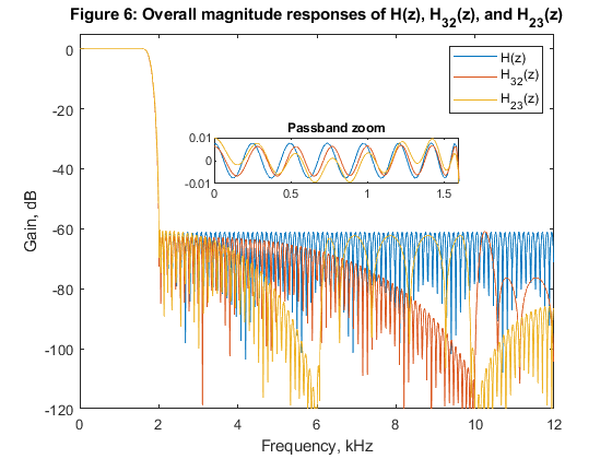
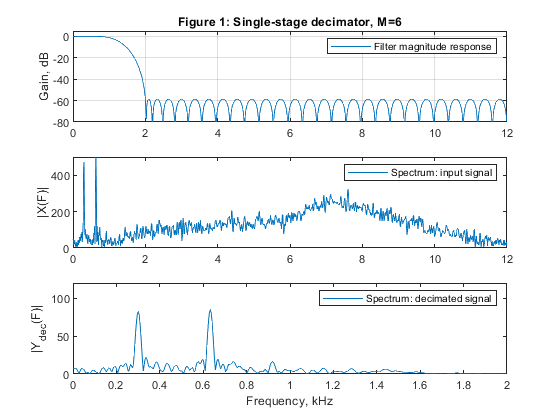
Exercise 4.6

Design and implement the factor-of-6 decimator, which converts the input frequency of 24 kHz to the frequency of 4 kHz.
a)   Design and implement the single-stage decimator.
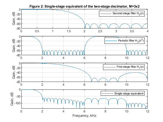
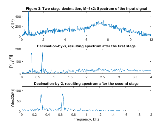
b)   Design and implement two-stage decimator with M₁ = 3, and M₂ = 2.
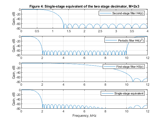
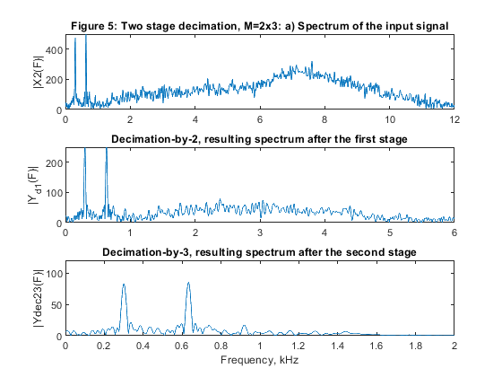
c)   Design and implement two-stage decimator with M₁ = 2, and M₂ = 3.
d)   Plot and comment on the results.
e)   Compute and compare the multiplication rates of the solutions from (a), (b) and (c).

Used functions: firpmord, firpm, fir2, freqz, upsample (Signal Processing Toolbox)

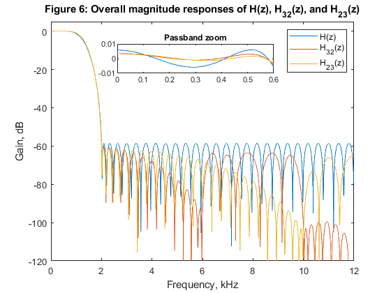
close all, clear all
% STEP a) Design and implementation of the factor-of-6 single-stage
% decimator.
% Lowpass FIR filter design, Case a tolerance scheme.
M = 6;                                                  % Decimation factor
ap = 0.01; as = 60; Fp = 0.05; Fs = 1/M;                % FIR filter design parameters
Fx = 24000;                                             % Sampling frequency (input)
dev = [(10^(ap/20)-1)/(10^(ap/20)+1),  10^(-as/20)];    % Passband and stopband ripples
F = [Fp Fs];                                            % Cutoff frequencies
A = [1 0];                                              % Desired amplitudes
[Nord,Fo,Ao,W]  = firpmord(F,A,dev);                    % Estimating the filter order
h = firpm(Nord,Fo,Ao,W);                                % Computing the filter coefficients
[H,F1] = freqz(h,1,1024,24);                            % Computation of filter frequency response
figure (1)
subplot(3,1,1), plot(F1,20*log10(abs(H))), legend('Filter magnitude response'), ylabel('Gain, dB')
title('Figure 1: Single-stage decimator, M=6')
axis([0,12,-80,5]),grid

Ndec1=Nord;

% Generating the input signal
n = 0:1008;                                              % Time index
ff = [0,0.2,0.5,0.6,0.8,1]; a = [0,0.3,0.5,0.9,0.4,0];
x = fir2(1008,ff,a);
x = 300*x+cos(2*pi*Fp/1.9*n)+cos(2*pi*Fp/4*n)+randn(size(n)); z=x;
[X,F1] = freqz(x,1,1024,24);                             % Computing the signal spectrum
subplot(3,1,2), plot(F1,abs(X)), legend('Spectrum: input signal'), ylabel('|X(F)|'), axis([0,12,0,500])
Fy=Fx/M;                                                 % Sampling frequency (output)

% Polyphase decomposition
E = reshape(h,6,length(h)/6);
% Polyphase downsampling and filtering
x0 = x(1:6:length(x)); x1 = [0,x(6:6:length(x))]; x2 = [0,x(5:6:length(x))];
x3 = [0,x(4:6:length(x))]; x4 = [0,x(3:6:length(x))]; x5 = [0,x(2:6:length(x))];
y0 = filter(E(1,:),1,x0); y1 = filter(E(2,:),1,x1); y2 = filter(E(3,:),1,x2); y3=filter(E(4,:),1,x3); y4=filter(E(5,:),1,x4); y5=filter(E(6,:),1,x5);
ydec = y0+y1+y2+y3+y4+y5; % Decimated signal
[Ydec,F2] = freqz(ydec,1,512,4);
subplot(3,1,3), plot(F2,abs(Ydec)), legend('Spectrum: decimated signal'), ylabel('|Y_d_e_c(F)|'), axis([0,2,0,120])
xlabel('Frequency, kHz')

% STEP b) Design and implementation of the two-stage decimator M = M1*M2, with M1 = 3, and M2 = 2
M1 = 3; M2 = 2;                                           % Decimation factors
ap1 = 0.01/2; as1 = 60;
Fp = 0.05; Fs = 1/M1;
Fp2 = 3*Fp;
Nord_h2 = 20;
h2 = firpm(Nord_h2,[0,Fp*3,1/M2,1],[1,1,0,0],[2*W(1),1]); % Second stage, designing filter H2(z)
[H2,F2] = freqz(h2,1,1024,8);                             % Frequency response of H2(z)
h2u = upsample(h2,3);                                     % Periodic filter H_2(z^3)
[H2u,F1] = freqz(h2u,1,1024,24);                          % Spectrum of the periodic filter H_2(z^3)
Nord_h1 = 11;
h1 = firpm(Nord_h1,[0,Fp,6.60/12,9.30/12],[1,1,0,0],[2*W(1),1]); % First stage, designing filter H1(z)
[H1,F1] = freqz(h1,1,1024,24);                            % Frequency response  of H1(z)
H32 = H1.*H2u;                                            % The overall frequency response
figure (2)
subplot(4,1,1), plot(F2,20*log10(abs(H2))), legend('Second-stage filter H_2(z)'), ylabel('Gain, dB'), axis([0,4,-80,2]),grid
title('Figure 2: Single-stage equivalent of the two-stage decimator, M=3x2')
subplot(4,1,2), plot(F1,20*log10(abs(H2u))),legend('Periodic filter H_2(z^3)'), ylabel('Gain, dB'),axis([0,12,-80,2]),grid
subplot(4,1,3), plot(F1,20*log10(abs(H1))), legend('First-stage filter H_1(z)'), ylabel('Gain, dB'), axis([0,12,-80,2]),grid
subplot(4,1,4), plot(F1,20*log10(abs(H32))), legend('Single-stage equivalent'), ylabel('Gain, dB'),xlabel('Frequency, kHz'),
grid

% Input signal
x1 = z;
[X1,F1] = freqz(x1,1,2048,24);                            % Spectrum of the input signal
figure (3)
subplot(3,1,1), plot(F1,abs(X1)), ylabel('|X1(F)|'), axis([0,12,0,500])
title('Figure 3: Two stage decimation, M=3x2: Spectrum of the input signal')

% Polyphase decomposition, M1 = 3
E1 = reshape(h1,3,length(h1)/3);
% Polyphase downsampling and filtering, M1 = 3
v0 = x(1:3:length(x)); v1 = [0,x(3:3:length(x))]; v2 = [0,x(2:3:length(x))];
y0 = filter(E1(1,:),1,v0); y1 = filter(E1(2,:),1,v1); y2 = filter(E1(3,:),1,v2);
yd1 = y0 + y1 + y2;                                        % Decimated signal
[Yd1,F12] = freqz(yd1,1,2048,8);
subplot(3,1,2), plot(F12,abs(Yd1)), ylabel('|Y_d_1(F)|'),
title('Decimation-by-3, resulting spectrum after the first stage')

% Polyphase decomposition, M2 = 2
h2=[h2,0];
E2 = reshape(h2,2,length(h2)/2);
% Polyphase downsampling and filtering, M2 = 2
x = yd1;
v0 = x(1:2:length(x)); v1 = [0,x(2:2:length(x))];
y0 = filter(E2(1,:),1,v0); y1 = filter(E2(2,:),1,v1);

ydec32 = y0 + y1;                                          % Decimated signal
[Ydec32,F3] = freqz(ydec32,1,2048,4);
subplot(3,1,3), plot(F3,abs(Ydec32)), ylabel('|Ydec32(F)|'), axis([0,2,0,120])
title('Decimation-by-2, resulting spectrum after the second stage')
xlabel('Frequency, kHz')

% STEP c) Design and implementation of the two-stage decimator M = M1*M2, with M1 = 2, and M2 = 3
M1 = 2; M2 = 3;                                           % Decimation factors
Nord_h3=6;
h3 = firpm(Nord_h3,[0,Fp,10.5/12,1],[1,1,0,0],[2*W(1),1]); % Filter H1(z)
h3=[h3,0];
[H3,F1] = freqz(h3,1,1024,24);                             % Frequency response  of H1(z)
Nord_h4=31;
h4 = firpm(Nord_h4,[0,2*Fp,1/M2,1],[1,1,0,0],[2*W(1),1]);  % Filter H2(z)
[H4,F2] = freqz(h4,1,1024,8);                              % Frequency response of H2(z)
h4u = upsample(h4,2);                                      % Periodic filter H_2(z^2)
[H4u,F1] = freqz(h4u,1,1024,24);                           % Spectrum of the periodic filter H_2(z^2)
H23 = H3.*H4u;                                             % The overall frequency response

figure (4)
subplot(4,1,1), plot(F2,20*log10(abs(H4))), legend('Second-stage filter H4(z)'),ylabel('Gain, dB'), axis([0,4,-80,2]),grid
title('Figure 4: Single-stage equivalent of the two stage decimator, M=2x3')
subplot(4,1,2), plot(F1,20*log10(abs(H4u))), legend('Periodic filter H4(z^2)'), ylabel('Gain, dB'),axis([0,12,-80,2]),grid
subplot(4,1,3), plot(F1,20*log10(abs(H3))), legend('First-stage filter H3(z)'), ylabel('Gain, dB'), axis([0,12,-80,2]),grid
subplot(4,1,4), plot(F1,20*log10(abs(H23))), legend('Single-stage equivalent'), ylabel('Gain, dB'), axis([0,12,-80,2]),grid
xlabel('Frequency, kHz')

% Input signal
x2=z;
[X2,F1] = freqz(x2,1,1024,24);                             % Computing the signal spectrum
figure (5)
subplot(3,1,1), plot(F1,abs(X2)), ylabel('|X2(F)|'), axis([0,12,0,500])
title('Figure 5: Two stage decimation, M=2x3: a) Spectrum of the input signal')

% Polyphase decomposition, M1 = 2
E1 = reshape(h3,2,length(h3)/2);
% Polyphase downsampling and filtering, M1 = 2
v0 = x2(1:2:length(x2)); v1 = [0,x2(2:2:length(x2))];
y0 = filter(E1(1,:),1,v0); y1 = filter(E1(2,:),1,v1);
yd1 = y0 + y1;                                             % Decimated signal
[Yd1,F22]=freqz(yd1,1,2048,12);
subplot(3,1,2), plot(F22,abs(Yd1)), ylabel('|Y_d_1(F)|'), axis([0,6,0,250])
title('Decimation-by-2, resulting spectrum after the first stage')

% Polyphase decomposition, M2 = 3
h4=[h4,0];
E2 = reshape(h4,3,length(h4)/3);
% Polyphase downsampling and filtering, M2 = 3
x = yd1;
v0 = x(1:3:length(x)); v1 = [0,x(3:3:length(x))]; v2 = [0,x(2:3:length(x))];
y0 = filter(E2(1,:),1,v0); y1 = filter(E2(2,:),1,v1); y2 = filter(E2(3,:),1,v2);

ydec23 = y0 + y1 + y2;                                    % Decimated signal
[Ydec23,F3] = freqz(ydec23,1,2048,4);
subplot(3,1,3), plot(F3,abs(Ydec23)), ylabel('|Ydec23(F)|'), axis([0,2,0,120])
title('Decimation-by-3, resulting spectrum after the second stage')
xlabel('Frequency, kHz')

% STEP e)
% Computing the multiplication rate for decimators designed in STEPS a),b) and c)
RM_6_dec1 = (Ndec1+1)*Fx/6;
RM1_3_dec2 = (Nord_h1+1)*Fx/3;
RM2_2_dec2 = 4*Fx/6;
RM_32_dec2 = RM1_3_dec2 + RM2_2_dec2;
RM1_2_dec3 = (Nord_h3+1)*Fx/2;
RM2_3_dec3 = (Nord_h4+1)*Fx/6;
RM_23_dec3 = RM1_2_dec3 + RM2_3_dec3;

figure (6)
plot(F1,20*log10(abs(H)), F1,20*log10(abs(H32)),F1,20*log10(abs(H23)))
xlabel('Frequency, kHz'),ylabel('Gain, dB'),axis([0,12,-120,5])
title('Figure 6: Overall magnitude responses of H(z), H_3_2(z), and H_2_3(z)')
legend('H(z)','H_3_2(z)','H_2_3(z)')
g(3)=axes('Position',[0.3 0.75 0.40 0.1]);
plot(F1(1:60),20*log10(abs(H(1:60))),F1(1:60),20*log10(abs(H32(1:60))),F1(1:60),20*log10(abs(H23(1:60))))
axis([0,0.6,-0.01,0.01]), title('Passband zoom')

% Comments
% Filters in this example have been designed to satisfy Case a tolerance
% scheme.
% Figure 6 displays the  magnitude responses of the single-stage equivalens
% for the three solutions considered in the example.
% Figures 1, 3, and 5 illustrate the succesful decimations in the cases of
% the single-stage decimator M = 6, and in the cases of the two-stage
% decimators M1 = 3, M2 = 2, and M1 = 2, M2 = 3.
% Filter complexities:
% a) Single-stage decimator M=6: Filter order 59
%    Multiplication rate: RM_6_dec1 = 240000 multiplications per second.
% b) Two-stage decimator M1=3, M2=2: Filter orders 11 and 20
%    Multiplication rate: RM_32_dec2 = 112000 multiplications per second.
% c) Two-stage decimator M1=2, M2=3: Filter orders 6 and 31
%    Multiplication rate RM_23_dec3 = 212000 multiplications per second.
% Evidently, the two-stage solution b) with M1 = 3, M2 = 2 exhibist the best
% multiplication rate.

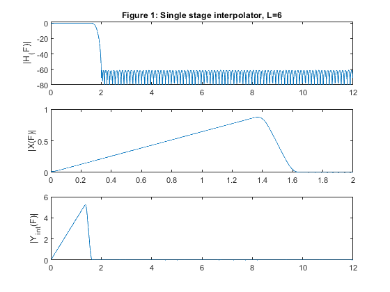
Exercise 4.7

Design and implement the factor-of-6 interpolator, which converts the input frequency of 4 kHz to the frequency of 24 kHz.
a)   Design and implement the single-stage dinterpolator.
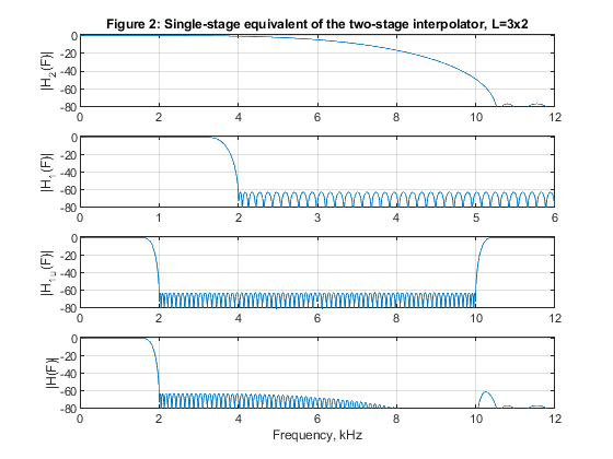
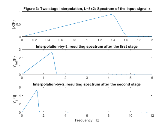
b)   Design and implement two-stage interpolator with L₁ = 3, and L₂ = 2.
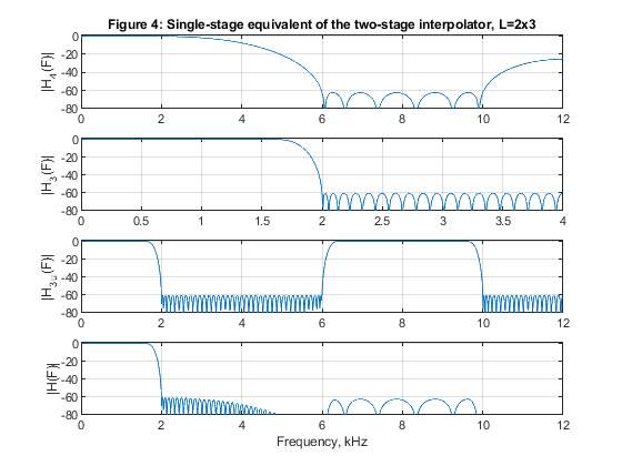
c)   Design and implement two-stage decimator with L₁ = 2, and L₂ = 3.
d)   Plot and comment on the results.
e)   Compute and compare the multiplication rates of the solutions from (a), (b) and (c).

Used functions: firpmord, firpm, fir2, freqz, upsample (Signal Processing Toolbox)

close all, clear all

% STEP a) Design and implementation of factor-of-6 single-stage interpolator
% Lowpass FIR filter design, Case a tolerance scheme.
L = 6;                                                         % Interpolation factor
ap = 0.01; as = 60; Fp = 1.6/12; Fs = 1/L;                     % FIR filter design parameters
Fx = 4000;                                                     % Sampling frequency (input)
Fy = L*Fx;                                                     % Sampling frequency (output)
dev = [(10^(ap/20)-1)/(10^(ap/20)+1);  10^(-as/20)];           % Passband and stopband ripples
F = [Fp Fs];                                                   % Cutoff frequencies
A = [1 0];                                                     % Desired amplitudes
[Nord,Fo,Ao,W]  = firpmord(F,A,dev);                           % Estimating the filter order
% We optimize the design parameters:
Nord=Nord-3; W=[1,1];
h = firpm(Nord,Fo,Ao,W);                                       % Filter H1(z)
[H,F1] = freqz(h,1,1024,24);                                   % Frequency response of H1(z)
figure (1)
subplot(3,1,1), plot(F1,20*log10(abs(H))), ylabel('|H_(F)|'), axis([0,12,-80,2])
title('Figure 1: Single stage interpolator, L=6');
L=6;
% Generating the input signal
ff = [0,0.7,0.8,1]; a = [0,0.9,0,0];
x = fir2(100,ff,a);
[X,F1] = freqz(x,1,1024,4);                                     % Spectrum of the input signal
figure (1)
subplot(3,1,2), plot(F1,abs(X)), ylabel('|X(F)|');

% Polyphase decomposition for the single stage with L=3
E = reshape(h,6,length(h)/6);

% Input to the interpolator L=6
% Poliphase filtering and up-sampling
u0 = L*filter(E(1,:),1,x); u1 = L*filter(E(2,:),1,x); u2 = L*filter(E(3,:),1,x);
u3 = L*filter(E(4,:),1,x); u4 = L*filter(E(5,:),1,x); u5 = L*filter(E(6,:),1,x);
U = [u0;u1;u2;u3;u4;u5];
yint = U(:); % interpolated signal
[Yint,F2] = freqz(yint,1,1024,24);
subplot(3,1,3), plot(F2,abs(Yint)), ylabel('|Y_i_n_t(F)|'), axis([0,12,0,6])

% STEP b) Design of two-stage factor-of-6 interpolator with L1=3 and L2=2.
h1 = firpm(103,[0,1.6/6,2/6,1],[1,1,0,0],[1,1]); % Filter H1(z)
h1 = [h1,0];
[H1,F1] = freqz(h1,1,1024,12);                                   % Frequency response of H1(z)
h2 = firpm(9,[0,1.6/12,10.5/12,1],[1,1,0,0],[5,1]); % Filter H2(F)
[H2,F2] = freqz(h2,1,1024,24);                                   % Frequency response of H2(z)
h1u = upsample(h1,2);                                            % Periodic filter H_1(z^2)
[H1u,F3] = freqz(h1u,1,1024,24);                                 % Spectrum of the periodic filter H_1(z^2)
H32 = H1u.*H2;                                                   % The overall frequency response
figure (2)
subplot(4,1,1), plot(F2,20*log10(abs(H2))), ylabel('|H_2(F)|'), axis([0,12,-80,2]),grid
title('Figure 2: Single-stage equivalent of the two-stage interpolator, L=3x2');
subplot(4,1,2), plot(F1,20*log10(abs(H1))), ylabel('|H_1(F)|'), axis([0,6,-80,2]),grid
subplot(4,1,3), plot(F3,20*log10(abs(H1u))), ylabel('|H_1_u(F)|'),axis([0,12,-80,2]),grid
subplot(4,1,4), plot(F2,20*log10(abs(H32))), ylabel('|H(F)|'), axis([0,12,-80,2]),grid
xlabel('Frequency, kHz')

L1 = 3; L2 = 2;
[X,F1] = freqz(x,1,1024,4);                                      % Spectrum of the input signal
figure (3)
subplot(3,1,1), plot(F1,abs(X)), ylabel('|X(F)|');
title('Figure 3: Two stage interpolation, L=3x2: Spectrum of the input signal x');

% Polyphase decomposition for the first stage with L1=3
h1=[h1];
E1 = reshape(h1,3,length(h1)/3);

% Input to the interpolator L1=3
% Poliphase filtering and up-sampling
u0 = L1*filter(E1(1,:),1,x); u1 = L1*filter(E1(2,:),1,x); u2 = L1*filter(E1(3,:),1,x);
U = [u0;u1;u2];
yint = U(:); % interpolated signal
[Yint,F3] = freqz(yint,1,1024,12);
subplot(3,1,2), plot(F3,abs(Yint)), ylabel('|Y_i_n_t(F)|'), axis([0,6,0,3])
title('Interpolation-by-3, resulting spectrum after the first stage')

% Polyphase decomposition for the second stage with L2=2
z=yint';
E2=reshape(h2,2,length(h2)/2);

% Input to the interpolator L2=2
% Poliphase filtering and up-sampling
v0 = L2*filter(E2(1,:),1,z); v1 = L2*filter(E2(2,:),1,z);
V = [v0;v1];
y = V(:);                                                        % Interpolated signal
[Y,F3] = freqz(y,1,2048,24);
subplot(3,1,3), plot(F3,abs(Y)); xlabel('Frequency, Hz'), ylabel('|Y_(F)|'), axis([0,12,0,6])
title('Interpolation-by-2, resulting spectrum after the second stage')

% STEP c) Design of two-stage factor-of-6 interpolator with L1=2 and L2=3.
h3 = firpm(68,[0,1.6/4,2/4,1],[1,1,0,0],[1.5,1]); % Filter H3(z)
[H3,F4] = freqz(h3,1,1024,8);                                   % Frequency response of H3(z)
h4 = firpm(18,[0,1.6/12,6/12,10/12],[1,1,0,0],[1.5,1]); % Filter H4(z)
[H4,F5] = freqz(h4,1,1024,24);                                  % Frequency response of H4(z)
h3u = upsample(h3,3);                                           % Periodic filter H_3(z^3)
[H3u,F6] = freqz(h3u,1,1024,24);                                % Spectrum of the periodic filter H_3(z^3)
H23 = H3u.*H4;                                                  % The overall frequency response
figure (4)
subplot(4,1,1), plot(F5,20*log10(abs(H4))), ylabel('|H_4(F)|'), axis([0,12,-80,2]),grid
title('Figure 4: Single-stage equivalent of the two-stage interpolator, L=2x3');
subplot(4,1,2), plot(F4,20*log10(abs(H3))), ylabel('|H_3(F)|'), axis([0,4,-80,2]),grid
subplot(4,1,3), plot(F6,20*log10(abs(H3u))), ylabel('|H_3_u(F)|'),axis([0,12,-80,2]),grid
subplot(4,1,4), plot(F5,20*log10(abs(H23))), ylabel('|H(F)|'), axis([0,12,-80,2]),xlabel('Frequency, kHz'),
grid

L1=2; L2=3;
[X,F1] = freqz(x,1,1024,4);                                     % Spectrum of the input signal
figure (5)
subplot(3,1,1), plot(F1,abs(X)), ylabel('|X(F)|');
title('Figure 5: Two-stage interpolation, L=3x2, spectrum of the input signal x');

% Polyphase decomposition for the first stage with L1=3
h3=[h3,0];
E1 = reshape(h3,2,length(h3)/2);

% Input to the interpolator L1=3
% Poliphase filtering and up-sampling
u0 = L1*filter(E1(1,:),1,x); u1 = L1*filter(E1(2,:),1,x);
U = [u0;u1];
yint = U(:);                                                    % Interpolated signal
[Yint,F3] = freqz(yint,1,1024,12);
subplot(3,1,2), plot(F3,abs(Yint)), ylabel('|Y_i_n_t(F)|'), axis([0,6,0,3])
title('Interpolation-by-2, resulting spectrum after the first stage')

% Polyphase decomposition for the second stage with L2=3
z=yint';
h4=[h4,0,0];
E2=reshape(h4,3,length(h4)/3);

% Input to the interpolator L2=3
% Poliphase filtering and up-sampling
v0 = L2*filter(E2(1,:),1,z); v1 = L2*filter(E2(2,:),1,z); v2 = L2*filter(E2(3,:),1,z);
V = [v0;v1;v2];
y = V(:);                                                       % Interpolated signal
[Y,F3] = freqz(y,1,2048,24);
subplot(3,1,3), plot(F3,abs(Y)); xlabel('Frequency, Hz'), ylabel('|Y_(F)|'), axis([0,12,0,6])
title('Interpolation-by-3, resulting spectrum after the second stage')

% STEP e) Computation of multiplication rates for three designed interpolators in STEPS 1), 2) and 3)
Nord_h = 185; Nord_h1 = 92; Nord_h2 = 5; Nord_h3 = 62; Nord_h4 = 9; Fy = 6*Fx;

RMint_6 = (Nord_h+1)*Fy/6;
RMint_32 = (Nord_h1+1)*Fy/6+(Nord_h2+1)*Fy/2;
RMint_23 = (Nord_h3+1)*Fy/6+(Nord_h4+1)*Fy/3;

figure (6)
F1 = F1*6;
plot(F1,20*log10(abs(H)), F1,20*log10(abs(H32)),F1,20*log10(abs(H23)))
xlabel('Frequency, kHz'),ylabel('Gain, dB'),axis([0,12,-120,5])
title('Figure 6: Overall magnitude responses of H(z), H_3_2(z), and H_2_3(z)')
legend('H(z)','H_3_2(z)','H_2_3(z)')
g(3)=axes('Position',[0.35 0.60 0.40 0.1]);
plot(F1(1:150),20*log10(abs(H(1:150))),F1(1:150),20*log10(abs(H32(1:150))),F1(1:150),20*log10(abs(H23(1:150))))
axis([0,1.6,-0.01,0.01]), title('Passband zoom')

% Comments
% Filters in this example have been designed to satisfy Case a tolerance
% scheme.
% Figure 6 displays the  magnitude responses of the single-stage equivalens
% for the three solutions considered in the example.
% Figures 1, 3, and 5 illustrate the succesful interpolations in the cases of
% the single-stage interpolator L=6, and in the cases of the two-stage
% interpolators L1=3, L2=2, and L1=2, L2=3.
% Filter complexities:
% 1. Single-stage interpolator L=6: Filter order 206
%    Multiplication rate: RM_6_int1 = 744000 multiplications per second
% 2. Two-stage interpolator M1=3, M2=2: Filter orders 103 and 9, respectively
%   Multiplication rate: RM_32_int2 = 444000 multiplications per second
% 3. Two-stage interpolator L1=2, L2=3: Filter orders 68 and 18,respectively
%   Multiplication rate RM_23_int3 =  332000 multiplications per second
% Evidently, the two-stage solution with L1=2, L2=3 exhibist the best
% multiplication rate.

Published with MATLAB® R2020b