Multirate Filtering for Digital Signal Processing: MATLAB® Applications, Chapter III: Filters in Multirate Systems - Exercises
Contents
Exercise 3.1
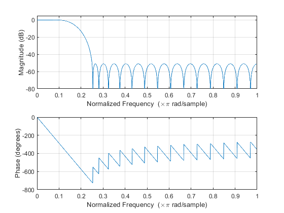
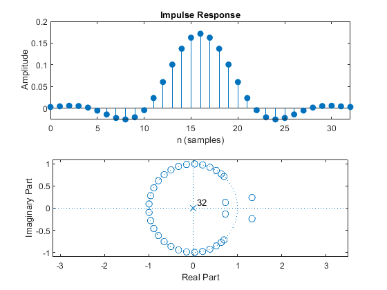
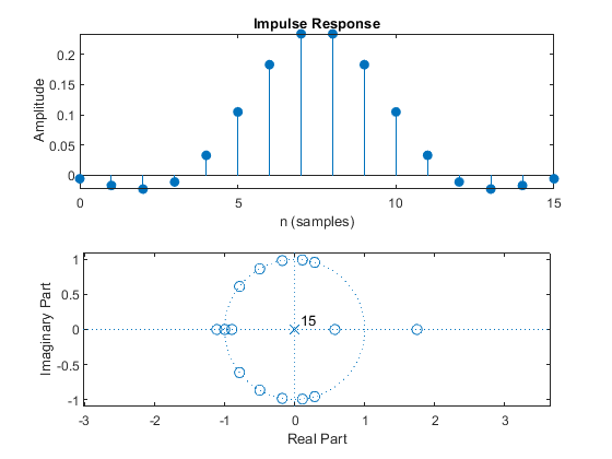
Design an optimal linear-phase FIR filter to satisfy the
Case a tolerance scheme of Figure 3.5 (a), for the sampling-rate
conversion factor M = 4.
The peak passband ripple is ap = 0.1 dB,
and the minimal stopband attenuation is as = 50 dB.
Choose the passband edge frequency ωp <π/M.
Compute and plot: impulse response, magnitude response, phase response, and pole-zero locations.
Used functions: firpmord, firpm (Signal Processing Toolbox)
clear all; close all;
M = 4;                                                  % Decimation factor M
ap = 0.1; as = 50; Fs = 1/M;                            % Filter specifications
% Fp = input('Choose the FIR filter passband edge frequency Fp<0.25: ');
Fp = 0.1;
dev = [(10^(ap/20)-1)/(10^(ap/20)+1),  10^(-as/20)];    % Passband and stopband ripples
F = [Fp Fs];                                            % Cutoff frequencies
A = [1 0];                                              % Desired amplitudes
[Nord,Fo,Ao,W] = firpmord(F,A,dev);                     % Estimating the filter order
Nord=Nord+0;                                            % Correction of the Nord when calculated value
% by firpmord function doesn't satisfy the Case a tolerance, so that designed filter fails to meet the requested stopband attenuation
h = firpm(Nord,Fo,Ao,W);                                % Filter coefficients based on Parks-McClellan algorithm
figure(1), freqz(h,1,1024),                             % Computes and plots the frequency response
axis([0,1,-80,5]), grid on;
figure(2),
subplot(2,1,1), impz(h,1);                              % Plots the impulse response
subplot(2,1,2), zplane(h,1);                            % Pole/zero plot
Exercise 3.2
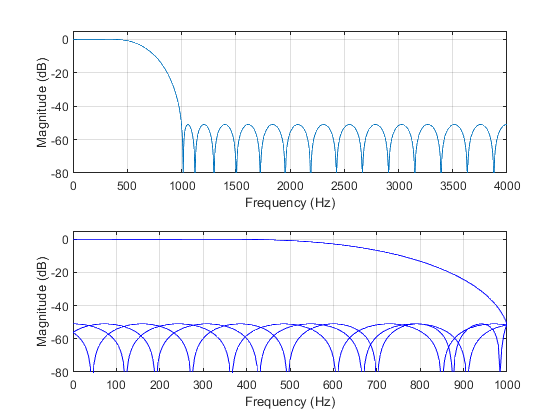
Compute and plot the aliasing characteristics of the 4-fold-decimator with
antialiasing filter from Exercise 3.1.
FIR filter: Coefficeints are computed by firpm function
according to the filter characteristics from Exercise 3.1.
Sampling frequencies: input Fx=8000 Hz, output Fy=2000 Hz.
Decimation factor M=4.
Used functions: firpmord, firpm (Signal Processing Toolbox)
clear all; close all;
M = 4;                                                  % Decimation factor
ap = 0.1; as = 50; Fs = 1/M;                            % Filter specifications
Fp = 0.1;
dev = [(10^(ap/20)-1)/(10^(ap/20)+1), 10^(-as/20)];     % Passband and stopband ripples
F = [Fp Fs];                                            % Cutoff frequencies
A = [1 0];                                              % Desired amplitudes
[Nord,Fo,Ao,W]  = firpmord(F,A,dev);                    % Estimating the filter order
h = firpm(Nord,Fo,Ao,W);                                % Filter coefficients
n = 0:length(h)-1;                                      % Time index
Fx = 8000;                                              % Input sampling frequency (Hz)
Fy = Fx/M;                                              % Output sampling frequency (Hz)
% Computing the filter magnitude response
for r=1:1001
    F(r) = (r-1)*Fx/2000;
    omega = 2*pi*F(r)/Fx;
    W = exp(-i*n*omega);
    H(r) = sum(h.*W);
end
figure(3),
subplot(2,1,1), plot(F,20*log10(abs(H))),
xlabel('Frequency (Hz)'), ylabel('Magnitude (dB)'),
axis([0,4000,-80,5]), grid

% Computing the unaliased characteristic and 4 aliased characteristics according to (3.30)
subplot(2,1,2),
k = 0;
for l=1:4
    for r=1:251
        FF(r) = (r-1)*Fy/500;
        omega = 2*pi*FF(r)/Fy;
        W = exp(-i*n*(omega-2*k*pi)/M);
        Hal(r) = sum(h.*W);
    end
    k = k + 1;
    plot(FF,20*log10(abs(Hal)),'b'), hold on,
end
xlabel('Frequency (Hz)'), ylabel('Magnitude (dB)'),
axis([0,1000,-80,5]), grid on, hold off;
Exercise 3.3
Design an optimal linear-phase FIR filter to satisfy the
Case b tolerance scheme of Figure 3.5 (b), for the sampling-rate
conversion factor M = 4.
The peak passband ripple is ap = 0.1 dB,
and the minimal stopband attenuation is as = 50 dB.
Choose the passband edge frequency ωp <
π/M.
Compute and plot: impulse response, magnitude response, phase response, and pole-zero locations.
Used functions: firpmord, firpm (Signal Processing Toolbox)
clear all; close all;
M=4;                                                    %Decimation factor M
ap = 0.1; as = 50;
%Fp = input('Choose the FIR filter passband edge frequency Fp<0.25: ');
Fp = 0.1;
Fs = 2/M-Fp;                                            % Filter specifications
dev = [(10^(ap/20)-1)/(10^(ap/20)+1),  10^(-as/20)];    % Passband and stopband ripples
F = [Fp Fs];                                            % Cutoff frequencies
A = [1 0];                                              % Desired amplitudes
[Nord,Fo,Ao,W]  = firpmord(F,A,dev);                    % Estimating the filter order
Nord = Nord+0;                                          %Correction of the Nord when calculated value doesn't satisfy the Case b tolerance
h = firpm(Nord,Fo,Ao,W);                                % Computing the filter coefficients
figure(1), freqz(h,1,1024),                             % Computes and plots the frequency response
axis([0,1,-80,5]);
figure(2),
subplot(2,1,1), impz(h,1);                              % Plots the impulse response
subplot(2,1,2), zplane(h,1);                            % Pole/zero plot

Exercise 3.4
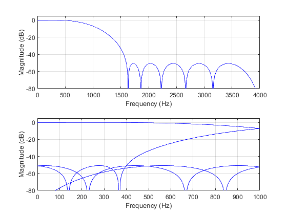
Compute and plot the aliasing characteristics of the 4-fold-decimator with
antialiasing filter from Exercise 3.3.
FIR filter: Coefficeints are computed by firpm
function according to the filter characteristics from Exercise 3.3.
Sampling frequencies: input Fx=8000 Hz, output Fy=2000 Hz. Decimation
factor M=4.
Used functions: firpmord, firpm (Signal Processing Toolbox)
clear all; close all;
M = 4;                                                  % Decimation factor
ap = 0.1; as = 50; Fp = 0.1; Fs = 2/M-Fp;               % Filter specifications
dev = [(10^(ap/20)-1)/(10^(ap/20)+1),  10^(-as/20)];    % Passband and stopband ripples
F = [Fp Fs];                                            % Cutoff frequencies
A = [1 0];                                              % Desired amplitudes
[Nord,Fo,Ao,W]  = firpmord(F,A,dev);                    % Estimating the filter order
h = firpm(Nord,Fo,Ao,W);                                % Filter coefficients
n = 0:length(h)-1;                                      % Time index
Fx = 8000;                                              % Input sampling frequency (Hz)
Fy = Fx/M;                                              % Output sampling frequency (Hz)
% Computing the filter magnitude response
for r=1:1001
    F(r) = (r-1)*Fx/2000;
    omega = 2*pi*F(r)/Fx;
    W = exp(-i*n*omega);
    H(r) = sum(h.*W);
end

figure(3),
subplot(2,1,1), plot(F,20*log10(abs(H)),'b'),
xlabel('Frequency (Hz)'),ylabel('Magnitude (dB)'),
axis([0,4000,-80,5]), grid;

% Computing the unaliased characteristic and 4 aliased characteristics according to (3.30)
subplot(2,1,2),
k = 0;
for l=1:4
    for r=1:251
        FF(r) = (r-1)*Fy/500;
        omega = 2*pi*FF(r)/Fy;
        W = exp(-i*n*(omega-2*k*pi)/M);
        Hal(r) = sum(h.*W);
    end
    k = k + 1;
    plot(FF,20*log10(abs(Hal)),'b'), hold on,
end
xlabel('Frequency (Hz)'),ylabel('Magnitude (dB)'),
axis([0,1000,-80,5]), grid on, hold off;
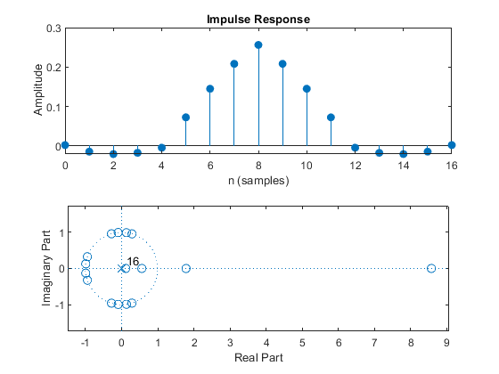
Exercise 3.5
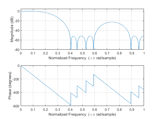
Design an optimal linear-phase FIR filter to satisfy the
Case c tolerance scheme of Figure 3.5 (c), for the sampling-rate
conversion factor M = 4.
The peak passband ripple is ap = 0.1 dB,
and the minimal stopband attenuation is as = 50 dB.
Choose the passband edge frequency ωp <
π/M.
Compute and plot: impulse response, magnitude response, phase response, and pole-zero locations.
Used functions: firpmord, firpm (Signal Processing Toolbox)
clear all; close all;
M = 4;                                                  %Decimation factor M
ap = 0.1; as = 50;                                      % Filter specifications
Fp = 0.1;
devp = (10^(ap/20)-1)/(10^(ap/20)+1);                   % Passband ripple
devs = 10^(-as/20);                                     % Stopband ripple
Fop = [0, Fp];                                          % Passband boundary frequencies
Fos1 = [2/M-Fp,2/M+Fp];                                 % Stopband 1 boundary frequencies
Fos2 = [4/M-Fp,min(4/M+Fp,1)];                          % Stopband 2 boundary frequencies
Fo= [Fop, Fos1, Fos2];                                  % Vector of normalized frequency points
Ao = [1,1,0,0,0,0];                                     % Desired amplitudes
W  = [1, devp/devs, devp/devs];                         % Estimating the filter order
Nord = 16;
h = firpm(Nord,Fo,Ao,W);                                % Computing the filter coefficients
figure(1),freqz(h,1,1024),                              % Computes and plots the frequency response
axis([0,1,-80,5]);
figure(2),
subplot(2,1,1),impz(h,1);                               % Plots the impulse response
subplot(2,1,2),zplane(h,1);                             % Pole/zero plot
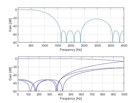
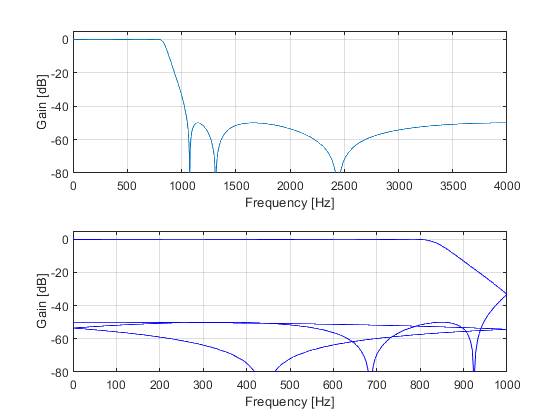
Exercise 3.6
Compute and plot the aliasing characteristics of the 4-fold-decimator with
antialiasing filter from Exercise 3.5.
FIR filter: Coefficeints are computed by firpm
function according to the filter characteristics from Exercise 3.5.
Sampling frequencies: input Fx=8000 Hz, output Fy=2000 Hz.. Decimation
factor M=4.
Used functions: firpmord, firpm (Signal Processing Toolbox)
clear all; close all;
M = 4;                                                  % Decimation factor
ap = 0.1; as = 50; Fp = 0.1;                            % Filter specifications
dev = [(10^(ap/20)-1)/(10^(ap/20)+1),  10^(-as/20)];    % Passband and stopband ripples
Fop = [0, Fp];                                          % Passband boundary frequencies
Fos1 = [2/M-Fp,2/M+Fp];                                 % Stopband 1 boundary frequencies
Fos2 = [4/M-Fp,min(4/M+Fp,1)];                          % Stopband 2 boundary frequencies
Fo= [Fop, Fos1, Fos2];                                  % Vector of normalized frequency points
Ao = [1,1,0,0,0,0];                                     % Desired amplitudes
W  = [1, dev(1)/dev(2), dev(1)/dev(2)];                 % Estimating the filter order
Nord = 16;
h = firpm(Nord,Fo,Ao,W);                                % Filter coefficients
n = 0:length(h)-1;                                      % Time index
Fx = 8000;                                              % Input sampling frequency (Hz)
Fy = Fx/M;                                              % Output sampling frequency (Hz)
% Computing the filter magnitude response
for r=1:1001
    F(r) = (r-1)*Fx/2000;
    omega = 2*pi*F(r)/Fx;
    W = exp(-i*n*omega);
    H(r) = sum(h.*W);
end

figure(3),
subplot(2,1,1),plot(F,20*log10(abs(H))),
xlabel('Frequency [Hz]'),ylabel('Gain [dB]'),
axis([0,4000,-80,5]),grid on;

% Computing the unaliased characteristic and 3 aliased characteristics according to (3.30)
subplot(2,1,2),
k = 0;
for l=1:4
    for r=1:251
        FF(r) = (r-1)*Fy/500;
        omega = 2*pi*FF(r)/Fy;
        W = exp(-i*n*(omega-2*k*pi)/M);
        Hal(r) = sum(h.*W);
    end
    k = k + 1;
    plot(FF,20*log10(abs(Hal)),'b'),hold on,
end
xlabel('Frequency [Hz]'),ylabel('Gain [dB]'),
axis([0,1000,-80,5]),grid on,hold off;
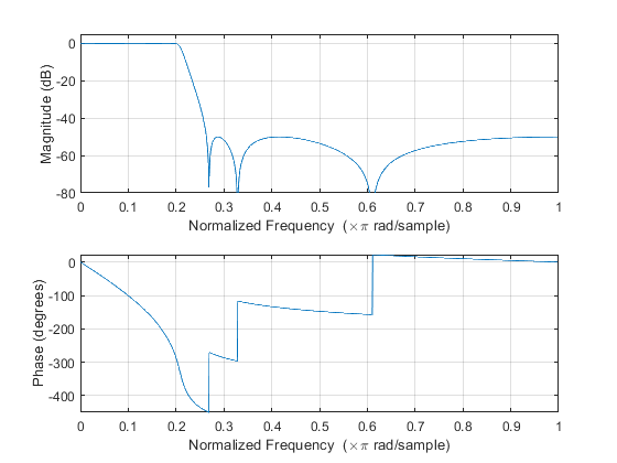
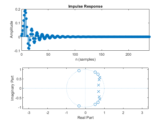
Exercise 3.7
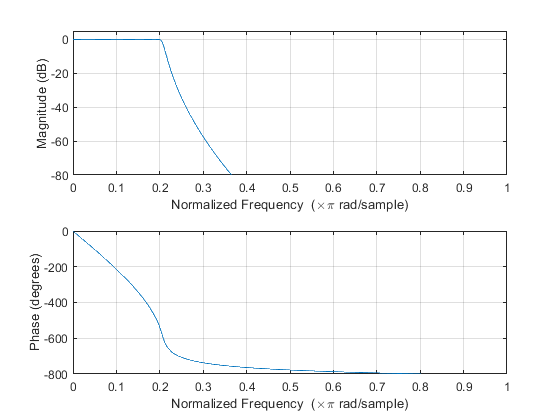
Design an elliptic IIR filter to satisfy the
Case b tolerance scheme of Figure 3.5 (b), for the sampling-rate
conversion factor M = 4.
The peak passband ripple is ap = 0.1 dB,
and the minimal stopband attenuation is as = 50 dB.
Choose the passband edge frequency ωp < π/M
.
Compute and plot: impulse response, magnitude response, phase response, and pole-zero locations.
Used functions: ellipord, ellip (Signal Processing Toolbox)
clear all; close all;
M=4;                                                    %Decimation factor M
ap = 0.1; as = 50;
Fp = 0.2;
Fs = 2/M-Fp;                                            % Filter specifications
dev = [(10^(ap/20)-1)/(10^(ap/20)+1),  10^(-as/20)];    % Passband and stopband ripples
F = [Fp Fs];                                            % Cutoff frequencies
[N,Fn] = ellipord(Fp,Fs,ap,as);                         % Estimating the filter order
[B,A] = ellip(N,ap,as,Fn);                              % Elliptic filter design
figure (1), freqz(B,A,1024),                            % Computes and plots the frequency response
axis([0,1,-80,5]),
figure (2),
subplot(2,1,1), impz(B,A);                              % Plots the impulse response of designed eliptic IIR filter
subplot(2,1,2), zplane(B,A);                            % Pole/zero plot
Exercise 3.8
Compute and plot the aliasing characteristics of
the 4-fold-decimator with IIR antialiasing filter from Exercise 3.7.
Sampling frequencies: input Fx=8000 Hz, output Fy=2000 Hz.
Decimation factor M=4.
Used functions: ellipord, ellip (Signal Processing Toolbox)
clear all;close all
M = 4;                                                  % Decimation factor
ap = 0.1; as = 50; Fp = 0.2; Fs = 2/M-Fp;               % Filter specifications
dev = [(10^(ap/20)-1)/(10^(ap/20)+1),  10^(-as/20)];    % Passband and stopband ripples
F = [Fp Fs];                                            % Cutoff frequencies
[N,Fn] = ellipord(Fp,Fs,ap,as);                         % Estimating the filter order
[B,A] = ellip(N,ap,as,Fn);                              % Elliptic filter design

[h,F]=impz(B,A);
n = (0:length(h)-1)';                                   % Time index
Fx = 8000;                                              % Input sampling frequency (Hz)
Fy = Fx/M;                                              % Output sampling frequency (Hz)
% Computing the filter magnitude response
for r=1:1001
    F(r) = (r-1)*Fx/2000;
    omega = 2*pi*F(r)/Fx;
    W = exp(-i*n*omega);
    H(r) = sum(h.*W);
end

figure(3),
subplot(2,1,1),plot(F,20*log10(abs(H))),
xlabel('Frequency [Hz]'),ylabel('Gain [dB]'),
axis([0,4000,-80,5]),grid on;

% Computing the unaliased characteristic and 3 aliased characteristics according to (3.30)
subplot(2,1,2),
k = 0;
for l=1:4
    for r=1:251
        FF(r) = (r-1)*Fy/500;
        omega = 2*pi*FF(r)/Fy;
        W = exp(-i*n*(omega-2*k*pi)/M);
        Hal(r) = sum(h.*W);
    end
    k = k + 1;
    plot(FF,20*log10(abs(Hal)),'b'),hold on,
end
xlabel('Frequency [Hz]'),ylabel('Gain [dB]'),
axis([0,1000,-80,5]),grid on,hold off;
Exercise 3.9
Design a Chebyshev IIR filter to satisfy the
Case b tolerance scheme of Figure 3.5 (b), for the sampling-rate
conversion factor M = 4.
The peak passband ripple is ap = 0.1 dB, and the minimal stopband attenuation is as = 50 dB. Choose the passband edge frequency
ωp < π/M.
Compute and plot: impulse response, magnitude response, phase response, and pole-zero locations.
Used functions: cheb1ord, cheby1 (Signal Processing Toolbox)
clear all; close all;
M=4;                                                    %Decimation factor M
ap = 0.1; as = 50;
Fp = 0.2;
Fs = 2/M-Fp;                                            % Filter specifications
dev = [(10^(ap/20)-1)/(10^(ap/20)+1),  10^(-as/20)];    % Passband and stopband ripples
F = [Fp Fs];                                            % Cutoff frequencies
[N,Fn] = cheb1ord(Fp,Fs,ap,as);                         % Estimating the filter order
[B,A] = cheby1(N,ap,Fn);                                % Chebyshev filter design
figure (1), freqz(B,A,1024),                            % Computes and plots the frequency response
axis([0,1,-80,5]),
figure (2),
subplot(2,1,1), impz(B,A);                              % Plots the impulse response of designed eliptic IIR filter
subplot(2,1,2), zplane(B,A);                            % Pole/zero plot

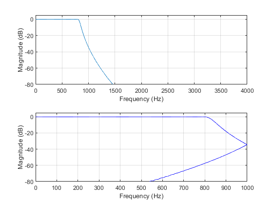
Exercise 3.10
Compute and plot the aliasing characteristics of
the 4-fold-decimator with IIR antialiasing filter from Exercise 3.9.
Sampling frequencies: input Fx=8000 Hz, output Fy=2000 Hz.
Decimation factor M=4.
Used functions: cheb1ord, cheby1 (Signal Processing Toolbox)
clear all; close all;
M = 4;                                                  % Decimation factor
ap = 0.1; as = 50; Fp = 0.2; Fs = 2/M-Fp;               % Filter specifications
dev = [(10^(ap/20)-1)/(10^(ap/20)+1),  10^(-as/20)];    % Passband and stopband ripples
F = [Fp Fs];                                            % Cutoff frequencies
[N,Fn] = cheb1ord(Fp,Fs,ap,as);                         % Estimating the filter order
[B,A] = cheby1(N,ap,Fn);                                % Chebyshev filter design

[h,F]=impz(B,A);
n = (0:length(h)-1)';                                   % Time index
Fx = 8000;                                              % Input sampling frequency (Hz)
Fy = Fx/M;                                              % Output sampling frequency (Hz)
% Computing the filter magnitude response
for r=1:1001
    F(r) = (r-1)*Fx/2000;
    omega = 2*pi*F(r)/Fx;
    W = exp(-i*n*omega);
    H(r) = sum(h.*W);
end

figure(3),
subplot(2,1,1), plot(F,20*log10(abs(H))),
xlabel('Frequency (Hz)'), ylabel('Magnitude (dB)'),
axis([0,4000,-80,5]), grid;

% Computing the unaliased characteristic and 4 aliased characteristics according to (3.30)
subplot(2,1,2),
k = 0;
for l=1:4
    for r=1:251
        FF(r) = (r-1)*Fy/500;
        omega = 2*pi*FF(r)/Fy;
        W = exp(-i*n*(omega-2*k*pi)/M);
        Hal(r) = sum(h.*W);
    end
    k = k + 1;
    plot(FF,20*log10(abs(Hal)),'b'), hold on,
end
xlabel('Frequency (Hz)'), ylabel('Magnitude (dB)'),
axis([0,1000,-80,5]), grid on, hold off;
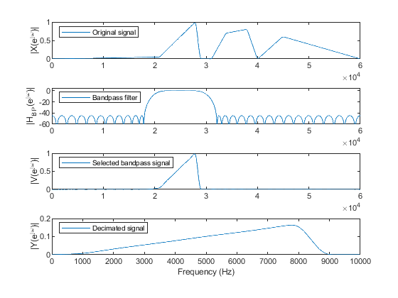
Exercise 3.11
Modify program demo_3_2 to study the integer-band decimation for the factor M = 6, and the input
sampling frequency of 120 kHz.
Select frequency band 20000-28000 kHz.
Used functions: downsample, fir2 (Signal Processing Toolbox), firgr (DSP System Toolbox)
clear all; close all;
Fx = 120000; M = 6; Fy = Fx/M;
F = [0,21000/60000,28000/60000,29000/60000,31000/60000,34000/60000,38000/60000,40000/60000,45000/60000,1];
A = [0,0.05,1,0,0,0.7,0.8,0,0.6,0];
x = fir2(511,F,A);                                          % Generating the input signal signal ‘x’
[X,f] = freqz(x,1,1024,Fx);                                 % Computing the spectrum of the signal ‘x’
figure(1),
subplot(4,1,1), plot(f,abs(X)), ylabel('|X(e^j^\omega)|');
legend('Original signal','Location','northwest')
% Setting the band pass filter to satisfy Eqs (3.32) and (3.33) for k =2.
ABp = [0,0,1,1,0,0];                                        % Desired magnitude response
FBp = [0,18000/60000,22000/60000,28000/60000,32000/60000,1];% Boundary frequencies
hBP = firgr(68,FBp,ABp); % Bandpass filter design
[HBP,f] = freqz(hBP,1,1024,Fx);                             % Computing the bandpass filter frequency response
subplot(4,1,2), plot(f,20*log10(abs(HBP))),
ylabel('|H_B_P(e^j^\omega)|'), axis([0,60000,-60,5]);
legend('Bandpass filter','Location','northwest')
v = filter(hBP,1,x);                                        % Bandpass filtering
[V,f] = freqz(v,1,1024,Fx);                                 % Computing the spectrum of the bandpass signal
subplot(4,1,3), plot(f,abs(V)),
ylabel('|V(e^j^\omega)|');
legend('Selected bandpass signal','Location','northwest')
y = downsample(v,M);                                        % Down-sampling of the bandpass signal
[Y,ff] = freqz(y,1,1024,Fy);                                % Computing the spectrum of the decimated signal
subplot(4,1,4); plot(ff,abs(Y)),
xlabel('Frequency (Hz)'), ylabel('|Y(e^j^\omega)|');
legend('Decimated signal','Location','northwest')
Exercise 3.12
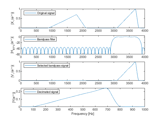
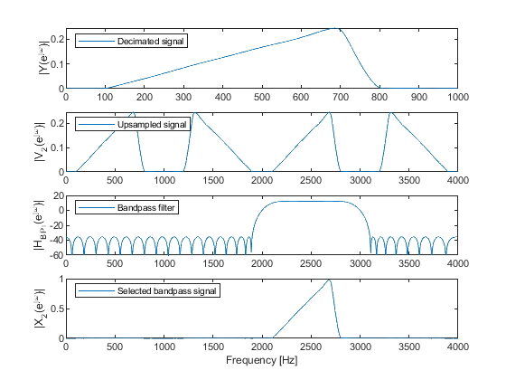
Using the integer-band decimation and the integer-band interpolation, develop the MATLAB program
which translates the selected band of frequencies into a desired position.
clear all; close all;
% This program is created to translate the bandpass signal from the range 3000 - 4000 Hz to the range 2000 - 3000 Hz.
% The sampling frequency is 8000 Hz, and conversion factors M = L =4.
Fx = 8000; M = 4; Fy = Fx/M;
F = [0,900/4000,1300/4000,1800/4000,2100/4000,2800/4000,3100/4000,3700/4000,3800/4000,1];
A = [0,0,0.3,0.7,0,0,0,1,0,0];
x1 = fir2(511,F,A);                                         % Generating the input signal signal ‘x’
[X1,f] = freqz(x1,1,1024,Fx);                               % Computing the spectrum of the signal ‘x’
figure(1),
subplot(4,1,1),
plot(f,abs(X1)),ylabel('|X_1(e^j^\omega)|'),
legend('Original signal','Location','northwest');
hBPd = firgr(68,[0,2900/4000,3100/4000,3700/4000,3900/4000,1],[0,0,1,1,0,0]); % Bandpass filter design
[HBPd,f] = freqz(hBPd,1,1024,Fx);                           % Computing the bandpass filter frequency response
subplot(4,1,2), plot(f,20*log10(abs(HBPd)))
legend('Bandpass filter','Location','northwest')
ylabel('|H_B_P_d(e^j^\omega)|'),axis([0,4000,-60,5]);
v1 = filter(hBPd,1,x1);                                     % Bandpass filtering
[V1,f] = freqz(v1,1,1024,Fx);                               % Computing the spectrum of the bandpass signal
subplot(4,1,3), plot(f,abs(V1)),ylabel('|V_1(e^j^\omega)|'),
legend('Selected bandpass signal','Location','northwest');
y = downsample(v1,M);                                       % Down-sampling of the bandpass signal
n = 0:length(y)-1;
y = y.*(-1).^n;                                             % Inverting the spectrum of the decimated signal (case k1=3, an odd number)
[Y,ff] = freqz(y,1,1024,Fy);                                % Computing the spectrum of the decimated signal
subplot(4,1,4); plot(ff,abs(Y)),
legend('Decimated signal','Location','northwest'),
ylabel('|Y(e^j^\omega)|'),xlabel('Frequency [Hz]');

% Integer-band interpolation (M=4, k2=2)
Fy = 2000; L = 4; Fz = 8000;
hBPi=L*firgr(64,[0,1900/4000,2200/4000,2800/4000,3100/4000,1],[0,0,1,1,0,0]); % Bandpass filter design
v2 = upsample(y,L);                                         % Up-sampling
[V2,f] = freqz(v2,1,1024,Fz);                               % Spectrum of the up-sampled signal
figure(2),
subplot(4,1,1),plot(ff,abs(Y)),ylabel('|Y(e^j^\omega)|'),
legend('Decimated signal','Location','northwest'),
subplot(4,1,2),plot(f,abs(V2)),ylabel('|V_2(e^j^\omega)|'),
legend('Upsampled signal','Location','northwest');
[HBPi,f] = freqz(hBPi,1,1024,Fz);                           % Computing the bandpass filter frequency response
subplot(4,1,3) ,plot(f,20*log10(abs(HBPi))),
ylabel('|H_B_P_i(e^j^\omega)|'),axis([0,4000,-60,20]);
legend('Bandpass filter','Location','northwest'),
x2 = filter(hBPi,1,v2);                                     % Filtering
[X2,f] = freqz(x2,1,1024,Fz);                               % Computing the spectrum of the bandpass interpolated signal
subplot(4,1,4), plot(f,abs(X2)),
ylabel('|X_2(e^j^\omega)|'),xlabel('Frequency [Hz]'),
legend('Selected bandpass signal','Location','northwest','Location','northwest');