Multirate Filtering for Digital Signal Processing: MATLAB® Applications, Chapter II: Basics of Multirate Systems - Exercises
Contents
Exercise 2.1
Generate the following sequences:
(i) sinusoidal sequence of normalized frequency 0.15
(ii) sum of two sinusoidal sequences of normalized frequencies 0.1 and 0.3
(iii) product of the sinusoidal sequence of normalized frequency 0.15 and the real exponential sequence {0.8n}.
Choose the sequence lengths to be 51.
a) Perform the factor-of-4 down-sampling. Plot the
original and down-sampled sequences.
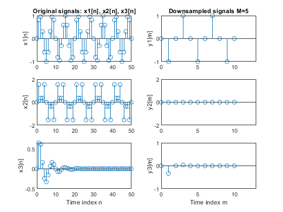
b) Repeat part (a) for the factor-of-5 down-sampler.
Used function: downsample (Signal Processing Toolbox)
clear all, close all
N = 51;                                 % Length of the sequences
n = 0:N-1;                              % Time index
x1 = sin(2*pi*0.15*n);                  % Signal x1-sinusoidal sequence of normalized frequency 0.15
x2 = sin(2*pi*0.1*n) + sin(2*pi*0.3*n); % Signal x2-sum of two sinusoidal sequences of normalized frequencies 0.1 and 0.3
x3 = x1.*0.8.^n; % Signal x3-product of the sinusoidal sequence of normalized frequency 0.15 and the real exponential sequence {0.8^n}

% (a)
M = 4;                                   % Down-sampling factor
y1 = downsample(x1,M);                   % Down-sampled signal y1
L1 = length(y1);                         % Length of the down-sampled sequence y1
y2 = downsample(x2,M);                   % Down-sampled signal y2
L2 = length(y2);                         % Length of the down-sampled sequence y2
y3 = downsample(x3,M);                   % Down-sampled signal y3
L3 = length(y3);                         % Length the down-sampled sequence y3
figure (1)
subplot(3,2,1), stem(0:N-1,x1(1:N)), ylabel('x1[n]');
title('Original signals x1[n], x2[n], x3[n]')
subplot(3,2,3), stem(0:N-1,x2(1:N)), ylabel('x2[n]');
subplot(3,2,5), stem(0:N-1,x3(1:N)), ylabel('x3[n]');
xlabel('Time index n')
subplot(3,2,2), stem(0:L1-1,y1(1:L1)), ylabel('y1[m]')
title('Downsampled signals M=4')
axis([0,13,-1,1])
subplot(3,2,4), stem(0:L2-1,y2(1:L2)), ylabel('y2[m]')
axis([0,13,-2,2])
subplot(3,2,6), stem(0:L3-1,y3(1:L3)), ylabel('y3[m]')
axis([0,13,-1,1])
xlabel('Time index m')

% (b)
M = 5;                                    % Down-sampling factor
y1 = downsample(x1,M);                    % Down-sampled signal y1 of x1
L1 = length(y1);                          % Length of the down-sampled sequence y1
y2 = downsample(x2,M);                    % Down-sampled signal y2 of x2
L2 = length(y2);                          % Length of the down-sampled sequence y2
y3 = downsample(x3,M);                    % Down-sampled signal y3 of x3
L3 = length(y3);                          % Length the down-sampled sequence y3
figure (2)
subplot(3,2,1), stem(0:N-1,x1(1:N)), ylabel('x1[n]');
title('Original signals: x1[n], x2[n], x3[n]')
subplot(3,2,3), stem(0:N-1,x2(1:N)), ylabel('x2[n]');
subplot(3,2,5), stem(0:N-1,x3(1:N)), ylabel('x3[n]');
xlabel('Time index n')
subplot(3,2,2), stem(0:L1-1,y1(1:L1)), ylabel('y1[m]')
title('Downsampled signals M=5')
axis([0,13,-1,1])
subplot(3,2,4), stem(0:L2-1,y2(1:L2)), ylabel('y2[m]')
axis([0,13,-2,2])
subplot(3,2,6), stem(0:L3-1,y3(1:L3)), ylabel('y3[m]')
axis([0,13,-1,1])
xlabel('Time index m')

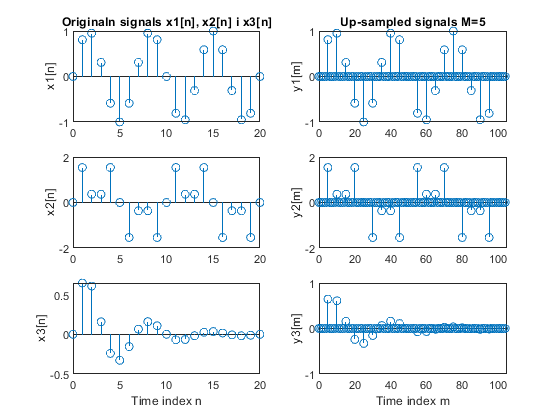
Exercise 2.2
Generate the following sequences:
(i) sinusoidal sequence of normalized frequency 0.15
(ii) sum of two sinusoidal sequences of normalized frequencies 0.1 and 0.3
(iii) product of the sinusoidal sequence of normalized frequency 0.15 and the real exponential sequence {0.8n}.
Choose the sequence lengths to be 21.
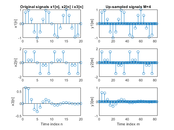
a) Perform the factor-of-4 up-sampling. Plot the
original and up-sampled sequences.
b) Repeat part (a) for the factor-of-5 up-sampler.
Used function: upsample (Signal Processing Toolbox)
clear all, close all;
N = 21;                                  % Length of the sequences
n = 0:N-1; % Time index
x1 = sin(2*pi*0.15*n);                   % Original signal x1-sinusoidal sequence of normalized frequency 0.15
x2 = sin(2*pi*0.1*n) + sin(2*pi*0.3*n);  % Original signal x2-sum of two sinusoidal sequences of normalized frequencies 0.1 and 0.3
x3 = x1.*0.8.^n; % Original signal x3-product of the sinusoidal sequence of normalized frequency 0.15 and the real exponential sequence {0.8^n}

% (a)
M = 4;                                   % Up-sampling factor
y1 = upsample(x1,M);                     % Up-sampled signal y1
L1 = length(y1);                         % Length of the up-sampled sequence y1
y2 = upsample(x2,M);                     % Up-sampled signal y2
L2 = length(y2);                         % Length of the up-sampled sequence y2
y3 = upsample(x3,M);                     % Up-sampled signal y3
L3 = length(y3);                         % Length of the up-sampled sequence y3
figure (1)
subplot(3,2,1), stem(0:N-1,x1(1:N)), ylabel('x1[n]');
title('Original signals x1[n], x2[n] i x3[n]')
subplot(3,2,3), stem(0:N-1,x2(1:N)), ylabel('x2[n]');
subplot(3,2,5), stem(0:N-1,x3(1:N)), ylabel('x3[n]');
xlabel('Time index n')
subplot(3,2,2), stem(0:L1-1,y1(1:L1)), ylabel('y1[m]')
title('Up-sampled signals M=4')
axis([0,L1,-1,1])
subplot(3,2,4), stem(0:L2-1,y2(1:L2)), ylabel('y2[m]')
axis([0,L2,-2,2])
subplot(3,2,6), stem(0:L3-1,y3(1:L3)), ylabel('y3[m]')
axis([0,L3,-1,1])
xlabel('Time index m')

% (b)
M = 5;                                   % Up-sampling factor
y1 = upsample(x1,M);                     % Up-sampled signal y1
L1 = length(y1);                         % Lengh of the up-sampled sequence y1
y2 = upsample(x2,M);                     % Up-sampled signal y2
L2 = length(y2);                         % Length of the up-sampled sequence y2
y3 = upsample(x3,M);                     % Up-sampled signal y3
L3 = length(y3);                         % Length of the up-sampled sequence y3
figure (2)
subplot(3,2,1), stem(0:N-1,x1(1:N)), ylabel('x1[n]');
title('Originaln signals x1[n], x2[n] i x3[n]')
subplot(3,2,3), stem(0:N-1,x2(1:N)), ylabel('x2[n]');
subplot(3,2,5), stem(0:N-1,x3(1:N)), ylabel('x3[n]');
xlabel('Time index n')
subplot(3,2,2), stem(0:L1-1,y1(1:L1)), ylabel('y1[m]')
title('Up-sampled signals M=5')
axis([0,L1,-1,1])
subplot(3,2,4), stem(0:L2-1,y2(1:L2)), ylabel('y2[m]')
axis([0,L2,-2,2])
subplot(3,2,6), stem(0:L3-1,y3(1:L3)), ylabel('y3[m]')
axis([0,L3,-1,1])
xlabel('Time index m')
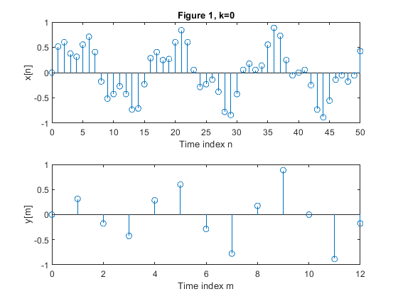
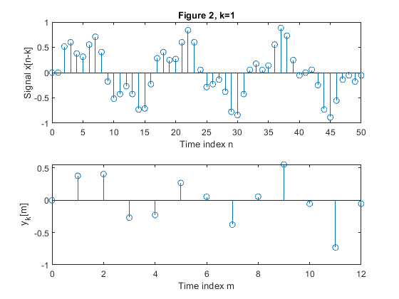
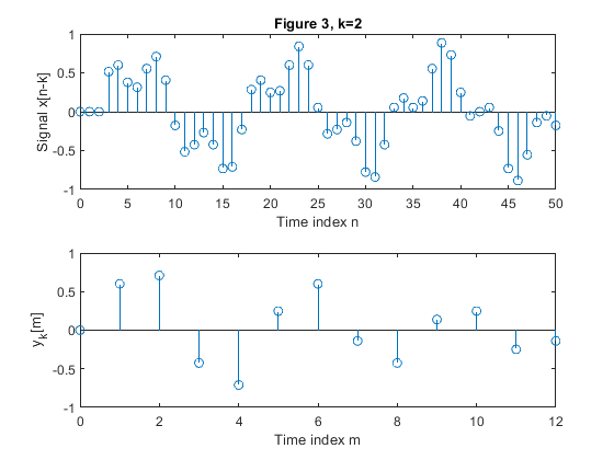
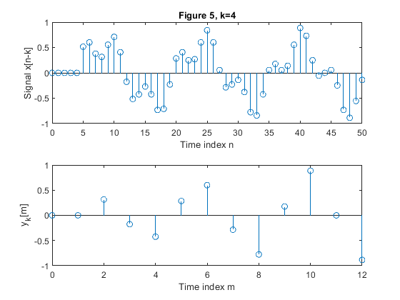
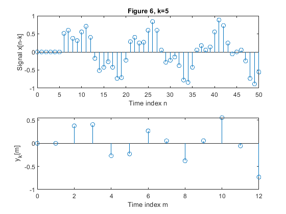
Exercise 2.3
Study the time-dependence property of the down-sampling operation on the example sequence {x[n]}.
{x[n]} is composed as a sum of two sinusoidal sequences of normalized frequencies 0.0625 and 0.2.
Choose N=51 for the sequence length.
Consider the sample values outside the interval {0,50} as zero valued.
With the conversion factor M = 4, down-sample the following sequences:
{x[n]}
{x[n-1]}
{x[n-2]}
{x[n-3]}
{x[n-4]}
{x[n-5]}
Plot the down-sampled sequences.
Used function: downsample (Signal Processing Toolbox)
clear all, close all;
N = 51;                                         % Length of the sequence
n = 0:N-1;                                      % Time index
x = 0.6*sin(2*pi*0.0625*n)+0.3*sin(2*pi*0.2*n); % Original signal
xp=zeros(N,1);
M = 4;                                          % Down-sampling factor
figure(1)
y = downsample(x,M);                            % Down-sampled signal x
L = length(y);                                  % Length of the down-sampled sequence
subplot(2,1,1), stem(0:N-1,x(1:N))
xlabel('Time index n'), ylabel('x[n]'),
title('Figure 1, k=0')
subplot(2,1,2)
stem(0:L-1,y(1:L))
xlabel('Time index m'), ylabel('y[m]')
for k=1:5,
    xk(1:k) = xp(1:k);
    xk(k+1:N) = x(1:(N-k));
    yk = downsample(xk,M);                       % Down-sampled signal x
    Lk = length(y);                              % Length of the down-sampled sequence
    figure(k+1)
    subplot(2,1,1), stem(0:N-1,xk(1:N))
    xlabel('Time index n'), ylabel(['Signal x[n-k]']) ,
    title(['Figure ' num2str(k+1) ', k=' num2str(k)]);
    subplot(2,1,2)
    stem(0:Lk-1,yk(1:Lk))
    xlabel('Time index m'), ylabel(['y_k[m]'])
end;

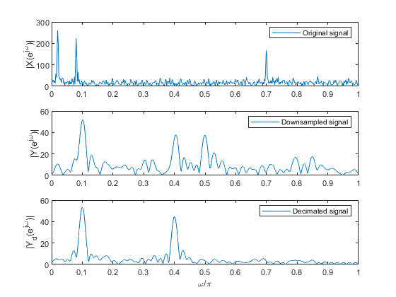
Exercise 2.4
Study the spectral characteristics of the down-sampled and decimated signals by modifying Program demo_2_3.
Generate 512 samples of the signal {x[n]}, composed of three sinusoidal sequences,
x[n]=sin(2πf1n)+0.9sin(2πf2n)+0.7sin(2πf3n)+0.8s[n]
where {s[n]} is the additive wideband noise of normal distribution,
which can be generated by using the MATLAB function randn.
Modify program demo_2_3 to compute and plot the spectra of
(i) original signal,
(ii) down-sampled-by-5 signal
(iii) decimated-by-5 signal.
Used functions: downsample, decimate (Signal Processing Toolbox).
clear all, close all;
% Input signal 'x'
N = 512;
n = 0:N-1;                                     % Time index n
f1 = 0.01;
f2 = 0.04;
f3 = 0.35;
x1 = sin(2*pi*f1*n)+0.9.*sin(2*pi*f2*n) + 0.7.*sin(2*pi*f3*n); %Generating the sinusoidal signal components
s = randn(1,N);
x = x1+0.8.*s;                                % Original signal
X = fft(x,1024);                              % Computing the spectrum of the original signal
f = 0:1/512:(512-1)/512;                      % Normalized frequencies
figure (1)
subplot(3,1,1), plot(f,abs(X(1:512)))
ylabel('|X(e^j^\omega)|'), legend('Original signal')
% Down-sampled signal
M = 5;                                       % Down-sampling factor
y = downsample(x,M);                         % Down-sampling
Y = fft(y,1024);                             % Computing the spectrum of the down-sampled signal
subplot(3,1,2), plot(f,abs(Y(1:512)))
ylabel('|Y(e^j^\omega)|'), legend('Downsampled signal')
% Decimated signal
yd = decimate(x,M);                          % Decimated-by-M signal
Yd = fft(yd,1024);                           % Computing the spectrum of the decimated signal
subplot(3,1,3), plot(f,abs(Yd(1:512)))
ylabel('|Y_d(e^j^\omega)|'), xlabel('\omega/\pi'), legend('Decimated signal')
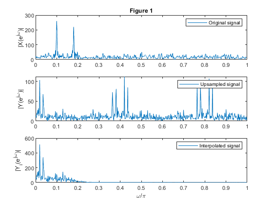
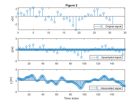
Exercise 2.5
Study the spectral characteristics of the
up-sampled and interpolated signals by modifying the Program demo_2_4.
Generate 512 samples of the signal {x[n]}, composed of two sinus.oidalasequences,
x[n]=sin(2π0.05n)+0.9sin(2π0.09n)+0.8s[n]
where {s[n]} is the additive wideband noise of normal distribution generated by using the MATLAB function randn.
Modify Program demo_2_4 to compute and plot the spectra of
(i) original signal,
(ii) up-sampled-by-5 signal,
(iii) interpolated-by-5 signal.
Used functions: upsample, interp (Signal Processing Toolbox).
clear all, close all;
% Input signal 'x'
N = 512;
n= 0:N-1;
f1 = 0.05;
f2 = 0.09;
x1 = sin(2*pi*f1*n)+0.9.*sin(2*pi*f2*n);           %Generating the signal components
s=randn(1,N);
x = x1+0.8.*s;                                     % Original signal
X = fft(x,1024);                                   % Computing the spectrum of the original signal
f = 0:1/512:(512-1)/512;                           % Normalized frequencies
figure (1)
subplot(3,1,1), plot(f,abs(X(1:512)))
ylabel('|X(e^j^\omega)|'), title('Figure 1'), legend('Original signal')
 % Up-sampled signal
M = 5;  % Up-sampling factor
y = upsample(x,M);                                 % Up-sampling
Y = fft(y,1024);                                   % Computing the spectrum of the up-sampled signal
subplot(3,1,2), plot(f,abs(Y(1:512)))
ylabel('|Y(e^j^\omega)|'), legend('Upsampled signal')
% Decimated signal
yi = interp(x,M);                                  % Interpolated-by-M signal
Yi = fft(yi,1024);                                 % Computing the spectrum of the interpolated-by-M signal
subplot(3,1,3), plot(f,abs(Yi(1:512)))
ylabel('|Y_i(e^j^\omega)|'), xlabel('\omega/\pi'), legend('Interpolated signal')

% Illustration of up-sampling and interpolation in time domain
figure (2)
subplot(3,1,1), stem(0:31,x(1:32))
ylabel('x[n]'), title ('Figure 2'), legend('Original signal','Location','southeast','NumColumns',4)
subplot(3,1,2), stem(M-1:M*32-1,y(M-1:M*32-1))
ylabel('y[m]'), legend('Upsampled signal','Location','southeast','NumColumns',4)
axis([M-1,M*32-1,-5,5])
subplot(3,1,3), stem(M-1:M*32-1,yi(M-1:M*32-1))
ylabel('y_i[m]'), xlabel('Time index'),legend('Interpolated signal','Location','southeast','NumColumns',4)
axis([M-1,M*32-1,-5,5])
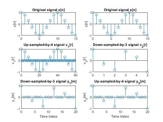
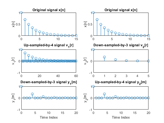
Exercise 2.6
Modify Program demo_2_7 to study the effects of the cascade interconnection of down-sampler and up-sampler.
Study the effects of interchanging positions of the down-sampler and the up-sampler
when converting sampling rate with rational factors:
(i) L/M = 4/3
(ii) L/M = 3/4.
Plot all sequences of interest, and comment on the results.
Generate the sequence x on your own choice, and repeat the procedure.
Used functions: downsample, upsample (Signal Processing Toolbox).
clear all, close all;
n = 0:15;                                        % Time index
L = 4; M = 3;                                    % Up-sampling and down-sampling factors
x = cos(0.2*pi*n);                               % Generating the original signal
v1 = upsample(x,L);                              % Up-sampling
y1 = downsample(v1,M);                           % Down-sampling
r = 0:length(v1)-1;                              % Time index
m = 0:length(y1)-1;                              % Time index
figure (1)
subplot(3,2,1), stem(n,x), ylabel('x[n]')
title('Original signal x[n]')
subplot(3,2,3), stem(r,v1), ylabel('v_1[r]')
title('Up-sampled-by-4 signal v_1[r]')
axis([0,60,-1,1])
subplot(3,2,5), stem(m,y1), ylabel('y_1[m]')
title('Down-sampled-by-3 signal y_1[m]'), axis([0,20,-1,1])
xlabel('Time Index')
v2 = downsample(x,M);                           % Down-sampling
r = 0:length(v2)-1;                             % Time index
y2 = upsample(v2,L);                            % Up-sampling
m = 0:length(y2)-1;                             % Time index
subplot(3,2,2), stem(n,x), ylabel('x[n]')
title('Original signal x[n]')
subplot(3,2,4), stem(r,v2), ylabel('v_2[r]')
title('Down-sampled-by-3 signal v_2[r]')
axis([0,5,-1,1])
subplot(3,2,6), stem(m,y2), ylabel('y_2[m]')
title('Up-sampled-by-4 signal y_2[m]'), xlabel('Time Index')
axis([0,20,-1,1])

n = 0:15;                                     % Time index
L = 4; M = 3;                                 % Up-sampling and down-sampling factors
x = 0.7.^n;                                   % Generating the original signal
v1 = upsample(x,L);                           % Up-sampling
y1 = downsample(v1,M);                        % Down-sampling
r = 0:length(v1)-1;                           % Time index
m = 0:length(y1)-1;                           % Time index
figure (2)
subplot(3,2,1), stem(n,x), ylabel('x[n]')
title('Original signal x[n]')
subplot(3,2,3), stem(r,v1), ylabel('v_1[r]')
title('Up-sampled-by-4 signal v_1[r]')
axis([0,60,-1,1])
subplot(3,2,5), stem(m,y1), ylabel('y_1[m]')
title('Down-sampled-by-3 signal y_1[m]'), axis([0,20,-1,1])
xlabel('Time Index')
v2 = downsample(x,M);                       % Down-sampling
r = 0:length(v2)-1;                         % Time index
y2 = upsample(v2,L);                        % Up-sampling
m = 0:length(y2)-1;                         % Time index
subplot(3,2,2), stem(n,x), ylabel('x[n]')
title('Original signal x[n]')
subplot(3,2,4), stem(r,v2), ylabel('v_2[r]')
title('Down-sampled-by-3 signal v_2[r]')
axis([0,5,-1,1])
subplot(3,2,6), stem(m,y2), ylabel('y_2[m]')
title('Up-sampled-by-4 signal y_2[m]'), xlabel('Time Index')
axis([0,20,-1,1])
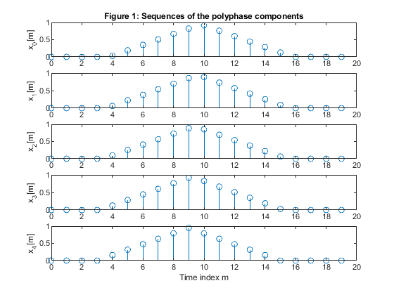
Exercise 2.7
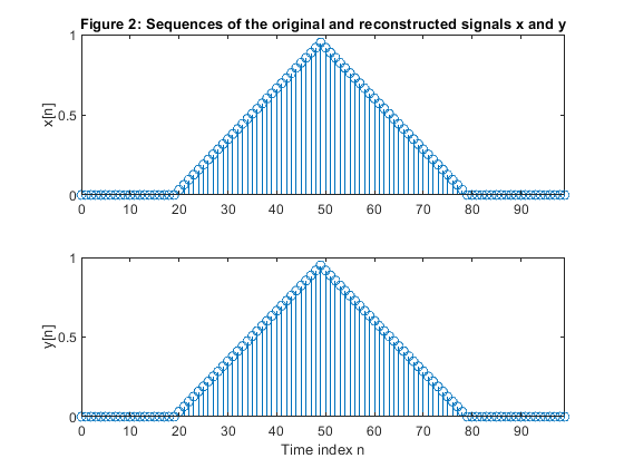
Generate the triangle-shape sequence of the length N = 100.
Perform the polyphase decomposition of the sequence for M = 5.
By modifying Program demo_2_9, perform the sequence reconstruction .
Plot the polyphase components.
Plot the original and the reconstructed sequences to demonstrate the exact reconstruction of the signal.
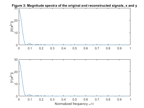
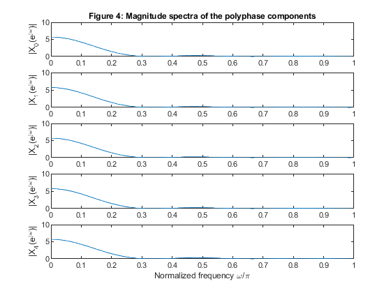
Compute and plot magnitude spectra of the original and reconstructed signals,
and also magnitude spectra of the polyphase components.
Used functions: downsample, upsample (Signal Processing Toolbox).
clear all, close all;
N=100;
n = 0:N-1;
x = zeros(size(n)); x(21:50) = (0.95.*(1:30))/30; x(51:80) = (0.95*30 - 0.95.*(1:30))/30;  % Generating the sequence ‘x’
M=5;
% Polyphase down-sampling with the phase offset
x0 = downsample(x,5);                          %Polyphase component x0
x1 = downsample(x,5,1);                        %Polyphase component x1
x2 = downsample(x,5,2);                        %Polyphase component x2
x3 = downsample(x,5,3);                        %Polyphase component x3
x4 = downsample(x,5,4);                        %Polyphase component x4

% Up-sampling polyphase components with the phase offset
y0 = upsample(x0,5);                           %Recomposed component y0
y1 = upsample(x1,5,1);                         %Recomposed component y1
y2 = upsample(x2,5,2);                         %Recomposed component y2
y3 = upsample(x3,5,3);                         %Recomposed component y3
y4 = upsample(x4,5,4);                         %Recomposed component y4

% Plot the polyphase components
figure (1)
subplot (5,1,1), stem(0:length(x0)-1,x0),ylabel('x_0[m]'), title('Figure 1: Sequences of the polyphase components')
subplot (5,1,2), stem(0:length(x1)-1,x1),ylabel('x_1[m]')
subplot (5,1,3), stem(0:length(x2)-1,x2),ylabel('x_2[m]')
subplot (5,1,4), stem(0:length(x3)-1,x3),ylabel('x_3[m]')
subplot (5,1,5), stem(0:length(x4)-1,x4),ylabel('x_4[m]')
xlabel('Time index m')

y = y0 + y1 + y2 + y3 +y4;                    % Adding together up-sampled polyphase components
% Plot the original and recomposed signals
figure (2)
subplot(2,1,1),stem(n,x), ylabel('x[n]'), axis([0,99,0,1]), title('Figure 2: Sequences of the original and reconstructed signals x and y')
subplot(2,1,2),stem(n,y), ylabel('y[n]'), axis([0,99,0,1])
xlabel('Time index n')

% Computing the magnitude spectra of the original and reconstructed signals
% and also the magnitude spectra of the polyphase components.
f = 0:1/500:(500-1)/500;
X = fft(x,1000);
Y = fft(y,1000);
f1 = 0:1/100:(100-1)/100;
X0 = fft(x0,200);
X1 = fft(x1,200);
X2 = fft(x2,200);
X3 = fft(x3,200);
X4 = fft(x4,200);

figure (3)
subplot (2,1,1), plot(f,abs(X(1:500))),ylabel('|X(e^j^\omega)|'), axis([0,1,0,30])
title('Figure 3: Magnitude spectra of the original and reconstructed signals, x and y')
subplot (2,1,2), plot(f,abs(Y(1:500))),ylabel('|Y(e^j^\omega)|'), axis([0,1,0,30])
xlabel('Normalized frequency \omega/\pi')
figure (4)
subplot (5,1,1), plot(f1,abs(X0(1:100))),ylabel('|X_0(e^j^\omega)|'), axis([0,1,0,10])
title('Figure 4: Magnitude spectra of the polyphase components')
subplot (5,1,2), plot(f1,abs(X1(1:100))),ylabel('|X_1(e^j^\omega)|'), axis([0,1,0,10])
subplot (5,1,3), plot(f1,abs(X2(1:100))),ylabel('|X_2(e^j^\omega)|'), axis([0,1,0,10])
subplot (5,1,4), plot(f1,abs(X3(1:100))),ylabel('|X_3(e^j^\omega)|'), axis([0,1,0,10])
subplot (5,1,5), plot(f1,abs(X4(1:100))),ylabel('|X_4(e^j^\omega)|'), axis([0,1,0,10])
xlabel('Normalized frequency \omega/\pi')
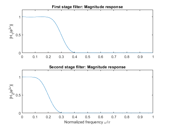
Exercise 2.8
Design FIR filters for the two-stage decimator,
which implements factor-of-15 sampling-rate conversion in two stages with M1 = 3 and M2 = 5.
Compute and plot magnitude responses of the two filters.
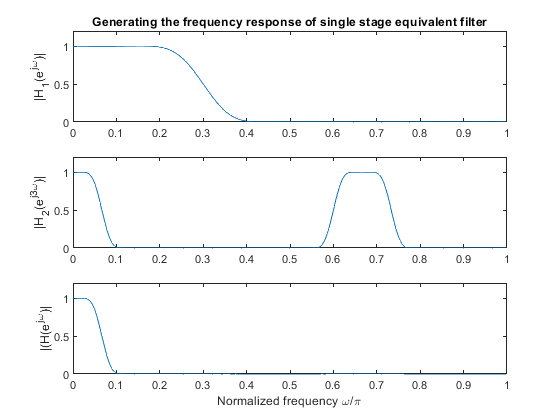
Compute frequency response of the equivalent filter for the single-stage decimator.
Plot the magnitude response of the equivalent single-stage filter.
Used functions: fir1, freqz (Signal Processing Toolbox)
clear all, close all;

h1 = fir1(30,0.3);                      % Designing FIR filter H1(z)
[H1,f] = freqz(h1,1,512,2);
figure (1)
subplot(2,1,1)
plot(f,abs(H1)), ylabel('|H_1(e^{j\omega})|'), title ('First stage filter: Magnitude response')
axis([0,1,0,1.2])

h2 = fir1(30,0.2);                      % Designing FIR filter H2(z)
[H2,f] = freqz(h2,1,512,2);
subplot(2,1,2)
plot(f,abs(H2)), ylabel('|H_2(e^{j\omega})|')
axis([0,1,0,1.2])
xlabel('Normalized frequency \omega/\pi'), axis([0,1,0,1.2]),title ('Second stage filter: Magnitude response')

% Computing the equivalent filter frequency response
M = 3;
h2u = zeros(1,M*length(h2));
h2u([1:M:length(h2u)]) = h2; % H2u(z) = H2(z^3)
[H2u,f] = freqz(h2u,1,512,2);

figure (2)
subplot(3,1,1)
plot(f,abs(H1)), ylabel('|H_1(e^{j\omega})|'), title('Generating the frequency response of single stage equivalent filter')
axis([0,1,0,1.2])
subplot(3,1,2), plot(f,abs(H2u)), ylabel('|H_2(e^{j3\omega})|')
axis([0,1,0,1.2])

H = H1.*H2u;                           % Equivalent filter
subplot(3,1,3), plot(f,abs(H)),ylabel('|(H(e^{j\omega})|')
xlabel('Normalized frequency \omega/\pi'), axis([0,1,0,1.2])