Multirate Filtering for Digital Signal Processing: MATLAB® Applications, Chapter XII: Examples of Multirate Filter Banks - Exercises
Contents
Exercise 12.1
Repeat the computations of Example 12.1.
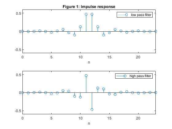
The impulse response of the linear-phase lowpass
FIR filter H0(z) is specified by vector B1,
which contains the first half of the filter coefficients,
B1=[0.002329266, -0.005182978, -0.002273145, 0.01354012, -0.0006504669, -0.02755195,
0.01004621, 0.05088162, -0.03464143, -0.09987885, 0.12464520,
0.4686479];
Generate and plot the new versions of Figures 12.4 – 12.6. Comment on the results.
Used functions: freqz (Signal Processing Toolbox)
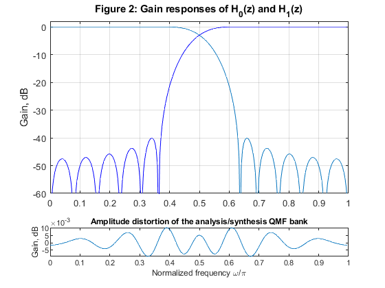
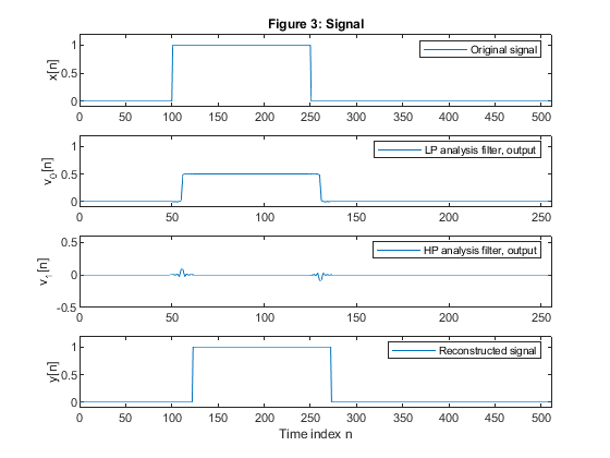
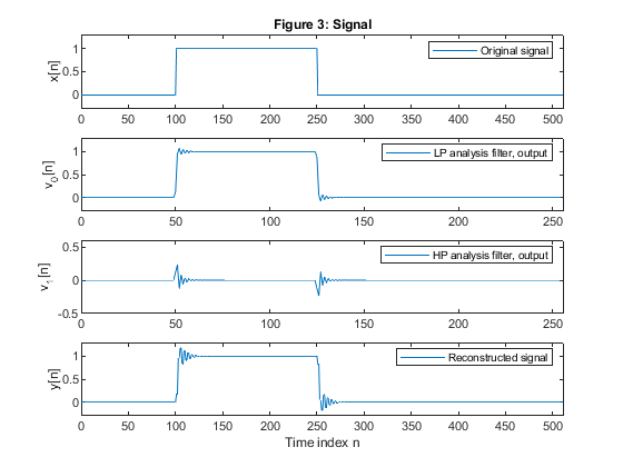
clear all,close all

 B1=[0.002329266,-0.005182978,-0.002273145,0.01354012,-0.0006504669,-0.02755195,...
  0.01004621,0.05088162,-0.03464143,-0.09987885,0.12464520,0.4686479];% filter length N=24

h0 = [B1,fliplr(B1)];                               % Generating the lowpass filter H0(z)
figure (1)
subplot(2,1,1)
stem(0:length(h0)-1,h0);title('Figure 1: Impulse response')
axis([0,23,-0.6,0.6]), xlabel('n'),
legend('low pass filter');
% Generate the complementary highpass filter

for k = 1:length(h0)                                % Generating the highpass filter H1(z)
   h1(k) = ((-1)^k)*h0(k);
end
figure (1)
subplot(2,1,2)
stem(0:length(h1)-1,h1);
axis([0,23,-0.6,0.6]), xlabel('n')
legend('high pass filter');
% Compute the gain responses of the two filters
[H1z,w]=freqz(h0,1,256);
H0=abs(H1z); g1=20*log10(H0);
[H2z,w]=freqz(h1,1,256);
H1=abs(H2z); g2=20*log10(H1);
% Plot the gain responses of the two filters
figure (2)
subplot(4,1,1:3)
plot(w/pi,g1,'-',w/pi,g2,'-b'),grid
title('Figure 2: Gain responses of H_0(z) and H_1(z)')
ylabel('Gain, dB')
axis([0,1,-60,2])

% Compute the sum of the square magnitude responses
ver=H0.^2+H1.^2;
figure (2)
subplot(5,1,5)
plot(w/pi,10*log10(ver))
xlabel('Normalized frequency \omega/\pi'), ylabel('Gain, dB')
title('Amplitude distortion of the analysis/synthesis QMF bank')

% Test signal
x = [zeros(size(1:100)),ones(size(101:250)),zeros(size(251:511))]; % Test signal

% Polyphase decomposition
e0 = h0(1:2:length(h0));                            % Polyphase component E_0(z)
e1 = h0(2:2:length(h0));                            % Polyphase component E_1(z)

% Analysis part
x0 = x(1:2:length(x))/2;                            % Down-sampling, branch E_0
x1 = [0,x(2:2:length(x)-1)]/2;                      % Down-sampling, branch E_1
v00 = filter(e0,1,x0);                              % Filtering with E_0(z)
v11 = filter(e1,1,x1);                              % Filtering with E_1(z)
v0 = v00 + v11;                                     % Output of the lowpass filter
v1 = v00 - v11;                                     % Output of the highpass filter

% Synthesis part
w00 = v0 + v1;                                      % Input to polyphase component E_1(z), synthesis part
w11 = v0 - v1;                                      % Input to polyphase component E_0(z), synthesis part
u00 = 2*filter(e1,1,w00);                           % Filtering with E_1(z)
u11 = 2*filter(e0,1,w11);                           % Filtering with E_0(z)
y0 = zeros(size(1:512));
y0(1:2:512) = u00;                                  % Upsampling, branch E_0
y1 = zeros(size(1:512));
y1(1:2:512) = u11;                                  % Upsampling, branch E_1
y0 = [0,y0(1:511)];                                 % Inserting the delay z^(-1)
y = 2*(y0 + y1);                                    % Reconstructed signal

figure (3)
subplot(4,1,1)
plot(1:511,x), ylabel('x[n]')
title('Figure 3: Signal')
axis([0,512,-0.1,1.2])
legend('Original signal')
subplot(4,1,2)
plot(0:255,v0),ylabel('v_0[n]')
axis([0,256,-0.1,1.2])
legend('LP analysis filter, output')
subplot(4,1,3)
plot(0:255,v1),ylabel('v_1[n]')
axis([0,256,-0.5,0.6])
legend('HP analysis filter, output')
subplot(4,1,4)
plot(0:511,y), xlabel('Time index n'), ylabel('y[n]')
legend('Reconstructed signal')
axis([0,512,-0.1,1.2])
Exercise 12.2
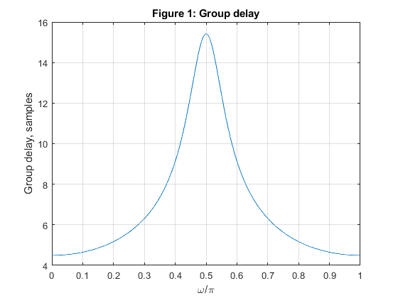
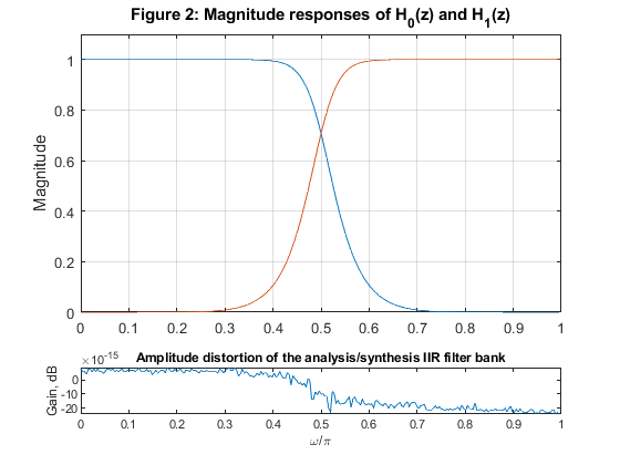
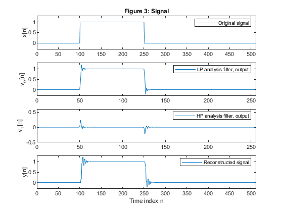
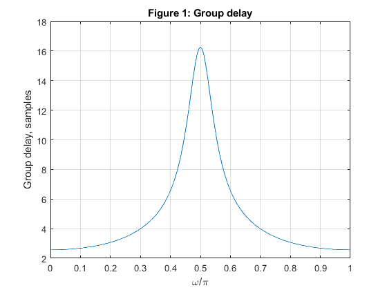
Repeat the computations of Example 12.2
using the 7th order Butterworth filter.
Generate and plot the new versions of Figures 12.8 – 12.10. Comment on the results.
Used functions: butter, grpdalay, freqz (Signal Processing Toolbox)
clear all, close all
N=7;                                                % Selecting the Butterworth filter order
[z,p,k]=butter(N,0.5);                              % Butterworth filter design
c=abs(p).^2;                                        % Squared moduli of the filter poles
g=sort(c(1:2:length(c)));
bet0=g(2:2:length(g));                              % Selecting beta coefficients for A0(z)
bet1=g(3:2:length(g));                              % Selecting beta coefficients for A1(z)

f=50/256;

% Composing the allpass branches A_0(z) and A_1(z)
P0=poly(-bet0);                                     % Allpass branch A_0(z)=Q0(z)/P0(z)
Q0=fliplr(P0);                                      % Allpass branch A_0(z)=Q0(z)/P0(z)
P1=poly(-bet1);                                     % Allpass branch A_1(z)=Q1(z)/P1(z)
Q1=fliplr(P1);                                      % Allpass branch A_1(z)=Q1(z)/P1(z)

TB = conv(upsample(Q0,2),upsample(Q1,2));
TB = [0,TB];
TA = conv(upsample(P0,2),upsample(P1,2));
[gd,f] = grpdelay(TB,TA,512,2);
figure (1)
plot(f,gd), grid, xlabel('\omega/\pi'),ylabel('Group delay, samples')
title('Figure 1: Group delay')

x = [zeros(size(1:100)),ones(size(101:250)),zeros(size(251:511))]; % Generating the test signal

% Analysis bank
xx=x/2;                                             % Scaling the input signal by 1/2
x0=xx(1:2:length(xx));                              % Down-sampling, branch A0
x1=[0,xx(2:2:length(xx))];                          % Down-sampling, branch A1
v00=filter(Q0,P0,x0);                               % Filtering with A_0(z)
v11=filter(Q1,P1,x1);                               % Filtering with A_1(z)
v0=v00+v11;                                         % Lowpass output
v1=v00-v11;                                         % Highpass output


% Synthesis bank
w00=v0+v1; % Input to A_0(z)
w11=v0-v1; % Input to B_0(z)
u00=filter(Q1,P1,w00);                              % Filtering with A_1(z)
u11=filter(Q0,P0,w11);                              % Filtering with A_0(z)
y0=zeros(size(1:512));
y0(1:2:512)=u00;                                    % Up-sampling, branch A_1
y1=zeros(size(1:512));
y1(1:2:512)=u11;                                    % Up-sampling, branch B_1
y0=[0,y0(1:511)];                                   % Inserting delay z^(-1)

y=y0+y1;                                            % Reconstructed signal

figure (2)
subplot(4,1,1:3)
B=k*poly(z); A=poly(p);                             % Lowpass filter H0(z)
[H0,f]=freqz(B,A,256,2);                            % Lowpass filter frequency response
plot(f,abs(H0))
hold on
BB=k*poly(-z);   AA = A;                            % Highpass filter H1(z)
[H1,f]=freqz(BB,AA,256,2);                          % Highpass filter frequency response
plot(f,abs(H1)),ylabel('Magnitude'), grid
axis([0,1,0,1.1])
title('Figure 2: Magnitude responses of H_0(z) and H_1(z)')
ver=abs(H0).^2+abs(H1).^2;
figure (2)
subplot(5,1,5)
plot(f,10*log10(ver))
xlabel('\omega/\pi'), ylabel('Gain, dB')
title('Amplitude distortion of the analysis/synthesis IIR filter bank')

figure (3)
subplot(4,1,1)
plot(1:511,x), ylabel('x[n]')
title('Figure 3: Signal')
axis([0,512,-0.3,1.3])
legend('Original signal')
subplot(4,1,2)
plot(0:255,v0),ylabel('v_0[n]')
axis([0,256,-0.3,1.3])
legend('LP analysis filter, output')
subplot(4,1,3)
plot(0:255,v1),ylabel('v_1[n]')
axis([0,256,-0.5,0.6])
legend('HP analysis filter, output')
subplot(4,1,4)
plot(0:511,y), xlabel('Time index n'), ylabel('y[n]')
legend('Reconstructed signal')
axis([0,512,-0.3,1.3])
Exercise 12.3
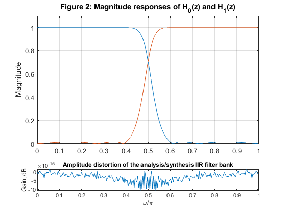
Repeat the computations of Example 12.2 using the 5th order elliptic filter
with the passband edge frequency
ωp=0.4π.
For the elliptic half-band IIR filter design use the MATLAB program halfbandiir given in Appendix A.
Generate and plot the new versions of Figures 12.8 – 12.10. Comment on the results.
Used functions: grpdalay, freqz (Signal Processing Toolbox), hallfbandiir (Appendix)
clear all, close all
N=5;                                                % Selecting the elliptic filter order
omega_p=0.4*pi;                                     % Angular passband edge frequency
fp=0.4;                                             % Passband edge frequency
[b,a,z,p,k]=halfbandiir(N,fp);                      % Elliptic filter design
c=abs(p).^2;                                        % Squared moduli of the filter poles
g=sort(c(1:2:length(c)));
bet0=g(2:2:length(g));                              % Selecting beta coefficients for A0(z)
bet1=g(3:2:length(g));                              % Selecting beta coefficients for A1(z)

f=50/256;

% Composing the allpass branches A_0(z) and A_1(z)
P0=poly(-bet0);                                     % Allpass branch A_0(z)=Q0(z)/P0(z)
Q0=fliplr(P0);                                      % Allpass branch A_0(z)=Q0(z)/P0(z)
P1=poly(-bet1);                                     % Allpass branch A_1(z)=Q1(z)/P1(z)
Q1=fliplr(P1);                                      % Allpass branch A_1(z)=Q1(z)/P1(z)

TB = conv(upsample(Q0,2),upsample(Q1,2));
TB = [0,TB];
TA = conv(upsample(P0,2),upsample(P1,2));
[gd,f] = grpdelay(TB,TA,512,2);
figure (1)
plot(f,gd), grid, xlabel('\omega/\pi'),ylabel('Group delay, samples')
title('Figure 1: Group delay')

x = [zeros(size(1:100)),ones(size(101:250)),zeros(size(251:511))]; % Generating the test signal

% Analysis bank
xx=x/2;                                             % Scaling the input signal by 1/2
x0=xx(1:2:length(xx));                              % Down-sampling, branch A0
x1=[0,xx(2:2:length(xx))];                          % Down-sampling, branch A1
v00=filter(Q0,P0,x0);                               % Filtering with A_0(z)
v11=filter(Q1,P1,x1);                               % Filtering with A_1(z)
v0=v00+v11;                                         % Lowpass output
v1=v00-v11;                                         % Highpass output


% Synthesis bank
w00=v0+v1;                                          % Input to A_0(z)
w11=v0-v1;                                          % Input to B_0(z)
u00=filter(Q1,P1,w00);                              % Filtering with A_1(z)
u11=filter(Q0,P0,w11);                              % Filtering with A_0(z)
y0=zeros(size(1:512));
y0(1:2:512)=u00;                                    % Up-sampling, branch A_1
y1=zeros(size(1:512));
y1(1:2:512)=u11;                                    % Up-sampling, branch B_1
y0=[0,y0(1:511)];                                   % Inserting delay z^(-1)

y=y0+y1;                                            % Reconstructed signal

figure (2)
subplot(4,1,1:3)
B=k*poly(z); A=poly(p);                             % Lowpass filter H0(z)
[H0,f]=freqz(B,A,256,2);                            % Lowpass filter frequency response
plot(f,abs(H0))
hold on
BB=k*poly(-z);   AA = A;                            % Highpass filter H1(z)
[H1,f]=freqz(BB,AA,256,2);                          % Highpass filter frequency response
plot(f,abs(H1)),ylabel('Magnitude'), grid
axis([0,1,0,1.1])
title('Figure 2: Magnitude responses of H_0(z) and H_1(z)')
ver=abs(H0).^2+abs(H1).^2;
figure (2)
subplot(5,1,5)
plot(f,10*log10(ver))
xlabel('\omega/\pi'), ylabel('Gain, dB')
title('Amplitude distortion of the analysis/synthesis IIR filter bank')

figure (3)
subplot(4,1,1)
plot(1:511,x), ylabel('x[n]')
title('Figure 3: Signal')
legend('Original signal')
axis([0,512,-0.3,1.3])
subplot(4,1,2)
plot(0:255,v0),ylabel('v_0[n]')
axis([0,256,-0.3,1.3])
legend('LP analysis filter, output')
subplot(4,1,3)
plot(0:255,v1),ylabel('v_1[n]')
axis([0,256,-0.5,0.6])
legend('HP analysis filter, output')
subplot(4,1,4)
plot(0:511,y), xlabel('Time index n'), ylabel('y[n]')
legend('Reconstructed signal')
axis([0,512,-0.3,1.3])
Example 12.4
Design the analysis/synthesis two-channel
orthogonal filter bank using the MATLAB function firpr2chfb.
The filter length is N=32, and the lowpass passband edge frequency
ωp=0.43π.
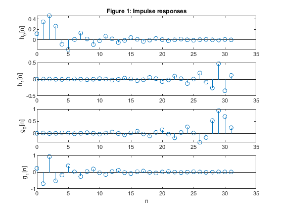
Plot the impulse responses of the analysis and synthesis filters: h0[n],
h1[n], g0[n] and
g1[n].
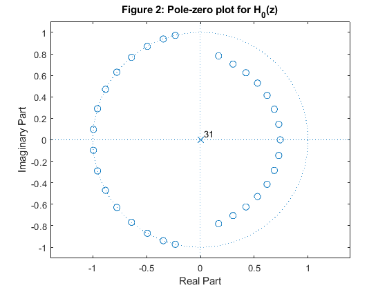
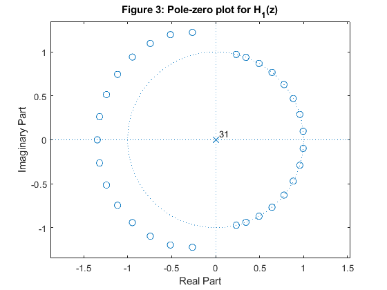
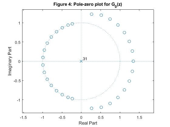
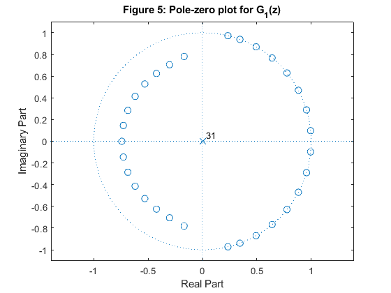
Compute and plot the poles and zeros of the transfer functions H0(z),
H1(z), G0(z) and
G1(z).
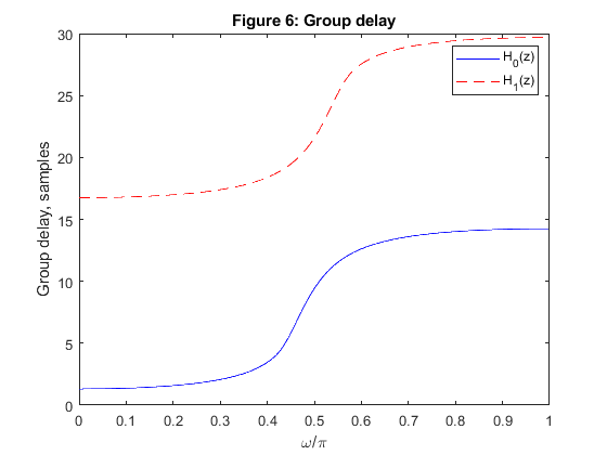
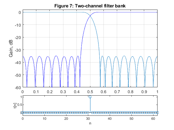
Compute and plot the magnitude and group delay responses of the analysis
filters H0(z) and
H1(z).
Compute and plot the impulse response of the distortion transfer function t[n]. Comment on the results.
Used functions: firpr2chfb, grpdelay, freqz (Signal Processing Toolbox)
clear all, close all
N = 32;
[h0,h1,g0,g1] = firpr2chfb(N-1,0.43);
n=0:N-1;
figure (1)
subplot(4,1,1)
stem(n,h0)
ylabel('h_0[n]')
title('Figure 1: Impulse responses')
subplot(4,1,2)
stem(n,h1)
ylabel('h_1[n]')
subplot(4,1,3)
stem(n,g0)
ylabel('g_0[n]')
subplot(4,1,4)
stem(n,g1)
ylabel('g_1[n]')
xlabel('n')
figure (2)
zplane(h0,1)
title('Figure 2: Pole-zero plot for H_0(z)')
figure (3)
zplane(h1,1)
title('Figure 3: Pole-zero plot for H_1(z)')
figure (4)
zplane(g0,1)
title('Figure 4: Pole-zero plot for G_0(z)')
figure (5)
zplane(g1,1)
title('Figure 5: Pole-zero plot for G_1(z)')
[Gdh0,f]=grpdelay(h0,1,512,2);
[Gdh1,f]=grpdelay(h1,1,512,2);
figure (6)
plot(f,Gdh0,'b',f,Gdh1,'--r')
xlabel('\omega/\pi'), ylabel('Group delay, samples')
title ('Figure 6: Group delay')
legend('H_0(z)','H_1(z)')
[H0,f]=freqz(h0,1,1024,2);
[H1,f]=freqz(h1,1,1024,2);
figure (7)
subplot(4,1,1:3)
plot(f,20*log10(abs(H0)),f,20*log10(abs(H1)),'b','LineWidth',1); grid
title('Figure 7: Two-channel filter bank')
xlabel('\omega/\pi'), ylabel('Gain, dB')
axis([0,1,-60,2])
figure(7)
subplot(4,1,4)
t = (conv(h0,g0)+conv(h1,g1))/2;
stem(0:2*(N-1),t)
xlabel('n'), ylabel('t[n]')
axis([0,2*(N-1),-0.2,1.1])
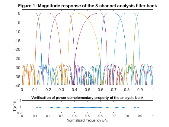
Example 12.5
Compose the eight-channel tree-structured
analysis/synthesis filter bank.
As a basic building block use the orthogonal two-channel filter bank of Example 12.4
and construct the analysis and synthesis banks.
Compute and plot the magnitude responses
of the resulting eight analysis filters.
Verify the magnitude-preserving property of the overall bank.
Comment on the phase characteristic of the overall analysis/synthesis bank.
Used functions firpr2chfb, upsample, freqz (Signal Processing Toolbox)
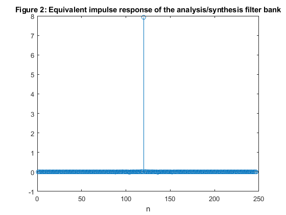
clear all, close all
N=18;
[h(1,:),h(2,:),g(1,:),g(2,:)]=firpr2chfb(N-1,0.4);  % MATLAB function for the analysis/synthesis orthogonal bank

% Analysis filters
r=1;
for k=1:2
    hh(r,:) = conv(h(k,:),upsample(h(1,:),2));      % Impulse response, 2nd level
    hh(r+1,:) = conv(h(k,:),upsample(h(2,:),2));    % Impulse response, 2nd level
    r=r+2;
end

r=1;
for k=1:4
    hhh(r,:) = conv(hh(k,:),upsample(h(1,:),4));    % Impulse response, 3rd level
    hhh(r+1,:) = conv(hh(k,:),upsample(h(2,:),4));  % Impulse response, 3rd level
    r=r+2;
end;

figure (1)
subplot(4,1,1:3)
for k=1:8
    [HHH(k,:),f]=freqz(hhh(k,:),1,1024,2);
    plot(f,20*log10(abs(HHH(k,:))))
    hold on
end
axis([0,1,-40,2])
title('Figure 1: Magnitude response of the 8-channel analysis filter bank')

% Verification of power complementary property of the analysis bank
Ver = zeros(size(1:1024));
for k=1:8
    HHH2(k,:)=abs(HHH(k,:));
    Ver = Ver + (HHH2(k,:)).^2;
end

figure (1),subplot(5,1,5)
plot(f,Ver);
xlabel('Normalized frequency \omega/\pi'),ylabel('|T(e^j^\omega)|')
title('Verification of power complementary property of the analysis bank')
axis([0,1,0.9,1.1])


% Equivalent 8-channel synthesis filter bank
r=1;
for k=1:2
    gg(r,:) = conv(g(k,:),upsample(g(1,:),2));
    gg(r+1,:) = conv(g(k,:),upsample(g(2,:),2));
    r=r+2;
end

r=1;
for k=1:4
    ggg(r,:) = conv(gg(k,:),upsample(g(1,:),4));
    ggg(r+1,:) = conv(gg(k,:),upsample(g(2,:),4));
    r=r+2;
end


for k=1:8
    t(k,:)=conv(hhh(k,:),ggg(k,:));
end

v=zeros(size(t(1,:)));
for k=1:8
    v=v+t(k,:);
end

figure (2)
stem(v)
title('Figure 2: Equivalent impulse response of the analysis/synthesis filter bank')
xlabel('n')

% Comment: The phase characteristic of the overall analysis/synthesis filter bank is linear.
% The equivalent impulse response of Figure 2 demonstrates the perfect reconstruction property,
% which can be achived if the overall filter bank exhibits a constant magnitude and linear phase response.
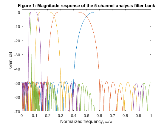
Example 12.6
Design an orthogonal two-channel FIR filter bank
with filter lengths of N=32.
Build the five-channel orthogonal analysis filter bank.
Develop the MATLAB program which computes the magnitude responses of the bank.
Used functions firpr2chfb, upsample, freqz (Signal Processing Toolbox)
clear all, close all
N=32;                                               % filter length
% We choose the passband edge frequency omega_p = 0.4*pi
[h0,h1,g0,g1]=firpr2chfb(N-1,0.4);                  % MATLAB function for the analysis/synthesis orthogonal bank

% Analysis filters: computing the equivalent impulse responses
r=2;
hb1 = h1;                                           % first level
hb2 = conv(h0,upsample(h1,2));                      % second level
hh = conv(h0,upsample(h0,2));
hb3 = conv(hh,upsample(h1,4));                      % third level
hh = conv(hh,upsample(h0,4));
hb4 = conv(hh,upsample(h1,8));                      % fourth level
hb5 = conv(hh,upsample(h0,8));                      % fourth level

[Hb(1,:),f] = freqz(hb1,1,1000,2);
[Hb(2,:),f] = freqz(hb2,1,1000,2);
[Hb(3,:),f] = freqz(hb3,1,1000,2);
[Hb(4,:),f] = freqz(hb4,1,1000,2);
[Hb(5,:),f] = freqz(hb5,1,1000,2);

figure (1)
for k=1:5
       plot(f,20*log10(abs(Hb(k,:))));
    hold on
end
axis([0,1,-70,2])
xlabel('Normalized frequency, \omega/\pi'),ylabel('Gain, dB')
title('Figure 1: Magnitude response of the 5-channel analysis filter bank')
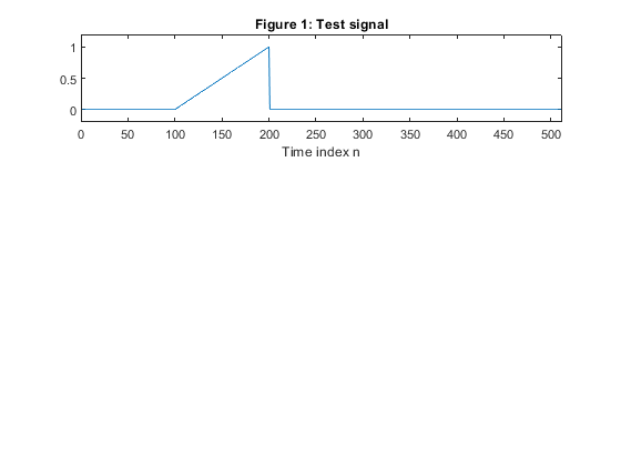
Exercise 12.7
Develop the MATLAB program for signal decomposition and reconstruction:
a) Using MATLAB function firpr2chfb design the analysis/synthesis two-channel
orthogonal filter bank for N=22 and fp=0.4.
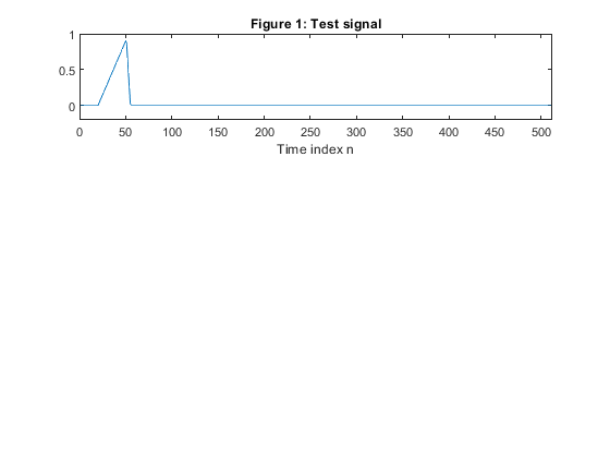
b) Generate the triangular-shape test signal.
c) Using the two-channel filter bank from (a),
construct the analysis four-level octave bank.
d) Perform the signal decomposition using the
four-level analysis filter bank.
e) Using the two-channel filter bank from (a),
construct the synthesis four-level octave bank.
f) Using the signal components from (d)
reconstruct the original signal.
g) Comment on the results.
Used functions firpr2chfb, upsample, downsample (Signal Processing Toolbox)
clear all
close all
% Analysis and synthesis octave bank

N =22;                                              % Setting the filter length
[h0,h1,g0,g1] = firpr2chfb(N-1,0.4);                % Designing the analysis/synthesis orthogonal two-channel filter bank

% Generating the test signal
x=[zeros(1,20),0.03*(1:30),0.03*(29:-7:1),zeros(1,511-55)];
figure (1)
subplot(3,1,1)
plot(x)
title('Figure 1: Test signal')
xlabel('Time index n')
axis([0,512,-0.2,1])

% Analysis bank
% Level 1
x0 = filter(h0,1,x);
x1 = filter(h1,1,x);
v0 = downsample(x0,2);
v1 = downsample(x1,2);

% Level 2
x2 = v0;
x02 = filter(h0,1,x2);
x12 = filter(h1,1,x2);
v02 = downsample(x02,2);
v12 = downsample(x12,2);
v2 = v12;

% Level 3
x3 = v02;
x03 = filter(h0,1,x3);
x13 = filter(h1,1,x3);
v03 = downsample(x03,2);
v13 = downsample(x13,2);
v3 = v13;

% Level 4
x4 = v03;
x04 = filter(h0,1,x4);
x14 = filter(h1,1,x4);
v04 = downsample(x04,2);
v14 = downsample(x14,2);
v4 = v14;
v5 = v04;


figure (2)
subplot(5,1,1)
plot(v1)
ylabel('v_1[n]'), title('Figure 2: Signal Analysis')
axis([0,256,-0.2,0.2])
subplot(5,1,2)
plot(v2)
ylabel('v_2[n]')
axis([0,256,-0.2,0.2])
subplot(5,1,3)
plot(v3)
ylabel('v_3[n]')
axis([0,256,-0.2,0.2])
subplot(5,1,4)
plot(v4)
ylabel('v_4[n]')
axis([0,256,-0.2,0.2])
subplot(5,1,5)
plot(v5)
ylabel('v_5[n]')
xlabel('Time index n')
axis([0,256,-0.2,1.2])


% Synthesis bank
% Level 4
w04=upsample(v5,2);
w14=upsample(v4,2);
y3=filter(g0,1,w04) + filter(g1,1,w14);

% Level 3
w13 = [zeros(size(1:N-1)),v3(1:length(v3)-(N-1))];
w13 = upsample(w13,2);
yu3 = upsample(y3,2);
y2 = filter(g0,1,yu3) + filter(g1,1,w13);

% Level 2
w12 = [zeros(size(1:3*(N-1))),v2(1:length(v2)-3*(N-1))];
w12 = upsample(w12,2);
yu2 = upsample(y2,2);
y1 = filter(g0,1,yu2) + filter(g1,1,w12);

% Level 1
w11 = [zeros(size(1:7*(N-1))),v1(1:length(v1)-7*(N-1))];
w11 = upsample(w11,2);
yu1 = upsample(y1,2);

y = filter(g0,1,yu1) + filter(g1,1,w11);            % Reconstructed signal

figure (3)
subplot(4,1,1)
plot(y3)
ylabel('y_3(n)'), title('Figure 3: Signal Synthesis')
axis([0,512,-0.2,1])
subplot(4,1,2)
plot(y2)
ylabel('y_2[n]')
axis([0,512,-0.2,1])
subplot(4,1,3)
plot(y1)
axis([0,512,-0.2,1])
ylabel('y_1[n]')
axis([0,512,-0.2,1.])
subplot(4,1,4)
plot(y)
ylabel('y[n]')
xlabel('Time index n')
axis([0,512,-0.2,1])
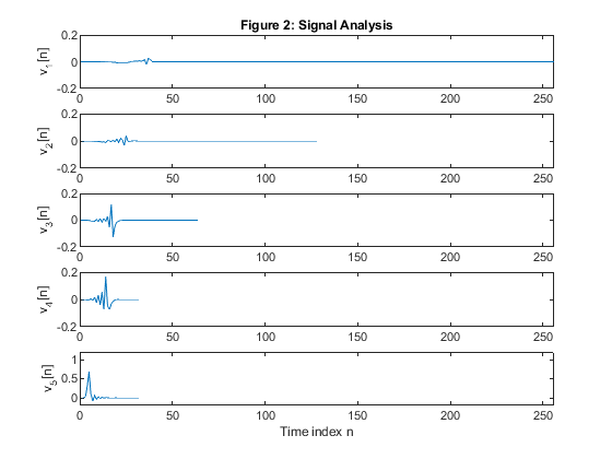

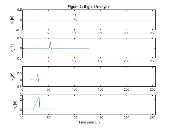
Exercise 12.8
Develop the MATLAB program for signal decomposition and reconstruction:
a) Design the two-channel analysis/synthesis bank using db5 wavelet filter.
b) Generate the triangular-shape test signal.
c) Using the two-channel filter bank from (a),
construct the analysis three-level octave bank.
d) Perform the signal decomposition using the
three-level analysis filter bank.
e) Using the two-channel filter bank from (a),
construct the synthesis three-level octave bank.
f) Using the signal components from (d)
reconstruct the original signal.
g) Comment on the results.
Used functions: wfilters (Wavelet Toolbox),downsample, upsample (Signal Processing Toolbox)
clear all
close all

wname = 'db5';                                      % Set wavelet name.
% Compute the four filters associated with wavelet name given by the input string wname.
[h0,h1,g0,g1] = wfilters(wname);
N = 10;                                             % The length of db5 filter

% Test signal
x=[zeros(size(1:100)),0.01*(1:100),zeros(size(201:511))];
figure (1)
subplot(3,1,1)
plot(x)
title('Figure 1: Test signal')
xlabel('Time index n')
axis([0,512,-0.2,1.2])

% Signal analysis
% Level 1
x0 = filter(h0,1,x);
x1 = filter(h1,1,x);
v0 = downsample(x0,2);
v1 = downsample(x1,2);

% Level 2
x2 = v0;
x02 = filter(h0,1,x2);
x12 = filter(h1,1,x2);
v02 = downsample(x02,2);
v12 = downsample(x12,2);
v2 = v12;

% Level 3
x3 = v02;
x03 = filter(h0,1,x3);
x13 = filter(h1,1,x3);
v03 = downsample(x03,2);
v13 = downsample(x13,2);
v3 = v13;
v4 = v03;

figure (2)
subplot(4,1,1)
plot(v1)
ylabel('v_1[n]'), title('Figure 2: Signal Analysis')
axis([0,256,-0.5,0.5])
subplot(4,1,2)
plot(v2)
ylabel('v_2[n]')
axis([0,256,-0.5,0.5])
subplot(4,1,3)
plot(v3)
ylabel('v_3[n]')
axis([0,256,-0.5,1])
subplot(4,1,4)
plot(v4)
ylabel('v_4[n]')
axis([0,256,-1,3])
xlabel('Time index, n')

% Signal synthesis
% Level 3
w03=upsample(v4,2);
Lw03=length(w03);
w13=upsample(v3,2);
Lw13=length(w13);
y2=filter(g0,1,w03) + filter(g1,1,w13);

% Level 2
w12 = [zeros(size(1:N-1)),v2(1:length(v2)-(N-1))];
Lw12=length(w12);
w12 = upsample(w12,2);
yu2 = upsample(y2,2);
y1 = filter(g0,1,yu2) + filter(g1,1,w12);

% Level 1
w11 = [zeros(size(1:3*(N-1))),v1(1:length(v1)-3*(N-1))];
w11 = upsample(w11,2);
yu1 = upsample(y1,2);
y1 = filter(g0,1,yu2) + filter(g1,1,w12);

y = filter(g0,1,yu1) + filter(g1,1,w11); % Reconstructed signal

figure (3)
subplot(3,1,1)
plot(y2)
ylabel('y_2(n)'), title('Figure 3: Signal Synthesis')
axis([0,512,-0.4,3.4])
subplot(3,1,2)
plot(y1)
ylabel('y_1[n]')
axis([0,512,-0.4,2.4])
subplot(3,1,3)
plot(y)
axis([0,512,-0.2,1.2])
ylabel('y[n]')
axis([0,512,-0.4,2.4])
xlabel('Time index, n')

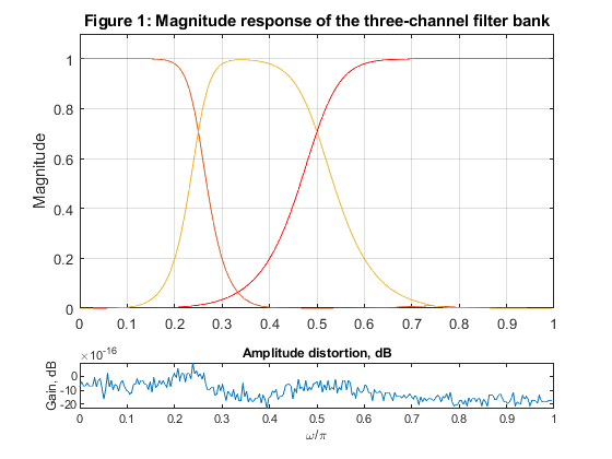
Exercise 12.9
Develop the MATLAB program for signal decomposition and reconstruction:
a) Utilize the two-channel Butterworth filter bank of Example 12.2 to
construct the two-level three-channel IIR octave analysis bank.
b) Compute and plot the magnitude responses of the bank.
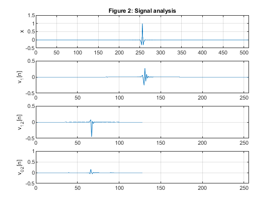
c) Utilize MATLAB program fir2 to generate the test signal with triangular shape spectrum.
d) Compute the signal components of the test signal as the outputs of the three-channel analysis bank.
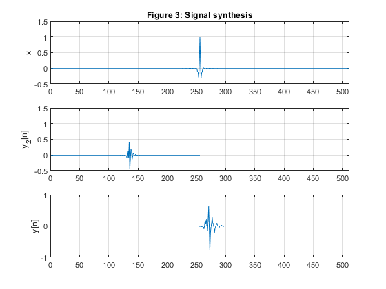
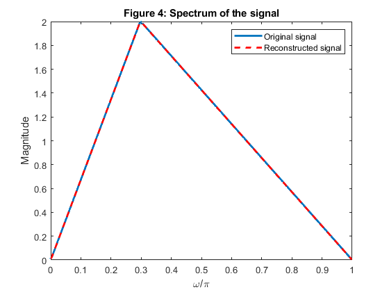
e) Construct the two-level three-channel synthesis bank and reconstruct the original test signal.
f) Comment on the results.
Used functions: butter, fir2, upsample, freqz (Signal Processing Toolbox)
clear all, close all
N=5;                                                % Selecting the Butterworth filter order
[z,p,k]=butter(N,0.5);                              % Butterworth filter design

subplot(4,1,1:3)
B=k*poly(z); A=poly(p);                             % Lowpass filter H0(z)
BB=k*poly(-z);   AA = A;                            % Highpass filter H1(z)
[H1,f]=freqz(BB,AA,256,2);                          % Highpass filter frequency response
[H0,f]=freqz(B,A,256,2);                            % Lowpass filter frequency response

figure (1)
plot(f,abs(H1),'r'),ylabel('Magnitude'), grid
hold on
B2=upsample(B,2);                                   % Lowpass filter, second level
BB2=upsample(BB,2);                                 % Highpass filter, second level
A2=upsample(A,2);
[H20,f]=freqz(B2,A2,256,2);                         % Lowpass filter frequency response,second level
[H21,f]=freqz(BB2,A2,256,2);                        % Highpass filter frequency response, second level
plot(f,abs(H0.*H20),f,abs(H0.*H21))
title('Figure 1: Magnitude response of the three-channel filter bank')
axis([0,1,0,1.1])

ver=abs(H0.*H20).^2+abs(H0.*H21).^2+abs(H1).^2;
figure (1)
subplot(5,1,5)
plot(f,2*log10(ver))
xlabel('\omega/\pi'), ylabel('Gain, dB')
title('Amplitude distortion, dB')
c=abs(p).^2;                                        % Squared moduli of the filter poles

g=sort(c(1:2:length(c)));
bet0=g(2:2:length(g));                              % Selecting beta coefficients for A0(z)
bet1=g(3:2:length(g));                              % Selecting beta coefficients for A1(z)

% Composing the allpass branches A_0(z) and A_1(z)
P0=poly(-bet0);                                     % Allpass branch A_0(z)=Q0(z)/P0(z)
Q0=fliplr(P0);                                      % Allpass branch A_0(z)=Q0(z)/P0(z)
P1=poly(-bet1);                                     % Allpass branch A_1(z)=Q1(z)/P1(z)
Q1=fliplr(P1);                                      % Allpass branch A_1(z)=Q1(z)/P1(z)

% Generating the test signal
x = fir2(510,[0,0.3,1],[0,2,0]);                    % Generating the test signal
[X,f]=freqz(x,1,1000);

% Analysis bank
% First level
xx=x/2;                                             % Scaling the input signal by 1/2
x0=xx(1:2:length(xx));                              % Down-sampling, branch A0
x1=[0,xx(2:2:length(xx))];                          % Down-sampling, branch A1
v00=filter(Q0,P0,x0);                               % Filtering with A_0(z)
v11=filter(Q1,P1,x1);                               % Filtering with A_1(z)
v0=v00+v11;                                         % Lowpass output
v1=v00-v11;                                         % Highpass output

% Second level
xx=v0/2;                                            % Scaling the input signal by 1/2
x0=[xx(1:2:length(xx))];                            % Down-sampling, branch A0
x1=[0,xx(2:2:length(xx))];                          % Down-sampling, branch A1
x1=x1(1:length(x1)-1);
v00=filter(Q0,P0,x0);                               % Filtering with A_0(z)
v11=filter(Q1,P1,x1);                               % Filtering with A_1(z)
v02=v00+v11;                                        % Lowpass output
v12=v00-v11;                                        % Highpass output

figure (2)
subplot(4,1,1)
plot(x),grid
ylabel('x')
axis([0,512,-0.5,1.5])
title('Figure 2: Signal analysis')
subplot(4,1,2)
plot(v1),grid
ylabel('v_1[n]')
axis([0,256,-0.5,0.5])
subplot(4,1,3)
plot(v12),grid
ylabel('v_1_2[n]')
axis([0,256,-0.5,0.5])
subplot(4,1,4)
plot(v02),grid
ylabel('v_0_2[n]')
axis([0,256,-0.5,1])

% Synthesis bank
% Second level
w02=v02+v12;                                        % Input to A_1(z)
w12=v02-v12;                                        % Input to A_0(z)
u00=filter(Q1,P1,w02);                              % Filtering with A_1(z)
u11=filter(Q0,P0,w12);                              % Filtering with A_0(z)
y0=zeros(size(1:256));
y0(1:2:256)=u00;                                    % Up-sampling, branch A_1
y1=zeros(size(1:256));
y1(1:2:256)=u11;                                    % Up-sampling, branch A_0
y0=[0,y0(1:255)];                                   % Inserting delay z^(-1)
y=y0+y1;
y2=y;

% First level
v1=filter(upsample(Q0,2),upsample(P0,2),v1);        % Postprocessing (v1), analysis part
v1=filter([0,upsample(Q1,2)],upsample(P1,2),v1);    % Preprocessing (v1), synthesis part


w00=y2+v1;                                          % Input to A_0(z)
w11=y2-v1;                                          % Input to B_0(z)
u00=filter(Q1,P1,w00);                              % Filtering with A_1(z)
u11=filter(Q0,P0,w11);                              % Filtering with A_0(z)
y0=zeros(size(1:512));
y0(1:2:512)=u00;                                    % Up-sampling, branch A_1
y1=zeros(size(1:512));
y1(1:2:512)=u11;                                    % Up-sampling, branch B_1
y0=[0,y0(1:511)];                                   % Inserting delay z^(-1)

y=y0+y1;                                            % Reconstructed signal

figure (3)
subplot(3,1,1)
plot(x),grid
title('Figure 3: Signal synthesis')
ylabel('x')
axis([0,512,-0.5,1.5])
subplot(3,1,2)
plot(y2),grid
ylabel('y_2[n]')
axis([0,512,-0.5,1.5])
subplot(3,1,3)
plot(y),grid
ylabel('y[n]')
axis([0,512,-1,1])

[Y,f]=freqz(y,1,1000,2);
figure (4)
plot(f,abs(X),'LineWidth', 2),grid
ylabel('Magnitude')
title('Figure 4: Spectrum of the signal')
hold on
plot(f,abs(Y),'--r','LineWidth', 2),grid
xlabel('\omega/\pi'),ylabel('Magnitude')
legend('Original signal', 'Reconstructed signal')

% Comment: Due to the perfect magnitude reconstruction property of the
% filter  bank, the analysis/synthesis bank exhibits the perfect
% reconstrucion of the magnitude spectrum of the input signal.