Multirate Filtering for Digital Signal Processing: MATLAB® Applications, Chapter XI: Filters in Multirate Systems - Exercises

Exercise 11.1
Exercise 11.2
Exercise 11.3
Exercise 11.4
Exercise 11.5
Exercise 11.6
Exercise 11.7

Exercise 11.1

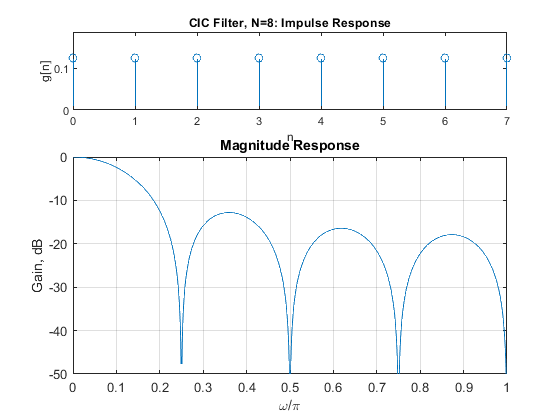
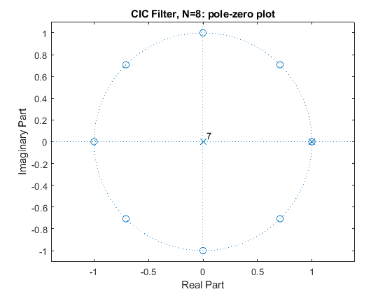
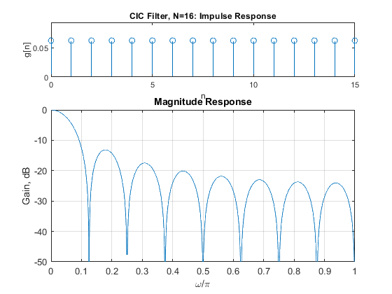
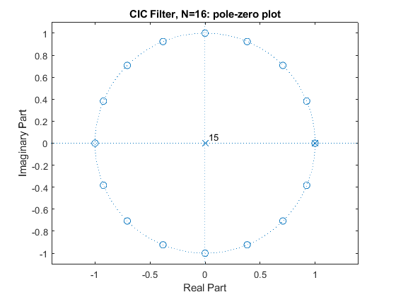
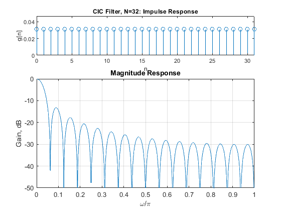
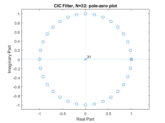
Compute and plot the impulse response, magnitude response, and the pole-zero plot of the single-stage CIC filters G(z) for N = 8, 16, and 32.

N=8;
g=rectwin(N)/N;                         % CIC filter impulse response
% Recursive representation of the CIC filter
% G(Z)=(1/N)*(1-z^(-N))/(1-z^-1)=(1/N)*B(z)/A(z)
B = [1,zeros(1,N-1),-1];
A = [1,-1];
[G,f]=freqz(B/N,A,1000,2);
figure(1),
subplot(3,1,1), stem(0:N-1,g), axis([0,N-1,0,(1+0.5)/N]),
xlabel('n'),ylabel('g[n]'),
title('CIC Filter, N=8: Impulse Response');
subplot(3,1,2:3),
plot(f,20*log10(abs(G))), xlabel('\omega/\pi'),ylabel('Gain, dB'),
title('Magnitude Response');
axis([0,1,-50,0]), grid,
figure(2),
zplane(B,A), title('CIC Filter, N=8: pole-zero plot');

N=16;
g=rectwin(N)/N;                                 % CIC filter impulse response
% Recursive representation of the CIC filter
% G(Z)=(1/N)*(1-z^(-N))/(1-z^-1)=(1/N)*B(z)/A(z)
B = [1,zeros(1,N-1),-1];
A = [1,-1];
[G,f]=freqz(B/N,A,1000,2);
figure(3),
subplot(3,1,1), stem(0:N-1,g), axis([0,N-1,0,(1+0.5)/N]),
xlabel('n'),ylabel('g[n]'),
title('CIC Filter, N=16: Impulse Response');
subplot(3,1,2:3),
plot(f,20*log10(abs(G))), xlabel('\omega/\pi'),ylabel('Gain, dB'),
title('Magnitude Response');
axis([0,1,-50,0]), grid,
figure(4),
zplane(B,A), title('CIC Filter, N=16: pole-zero plot');

N=32;
g=rectwin(N)/N;                                 % CIC filter impulse response
% Recursive representation of the CIC filter
% G(Z)=(1/N)*(1-z^(-N))/(1-z^-1)=(1/N)*B(z)/A(z)
B = [1,zeros(1,N-1),-1];
A = [1,-1];
[G,f]=freqz(B/N,A,1000,2);
figure(5),
subplot(3,1,1), stem(0:N-1,g), axis([0,N-1,0,(1+0.5)/N]),
xlabel('n'),ylabel('g[n]'),
title('CIC Filter, N=32: Impulse Response');
subplot(3,1,2:3),
plot(f,20*log10(abs(G))), xlabel('\omega/\pi'),ylabel('Gain, dB'),
title('Magnitude Response');
axis([0,1,-50,0]), grid,
figure(6),
zplane(B,A), title('CIC Filter, N=32: pole-zero plot');

Exercise 11.2

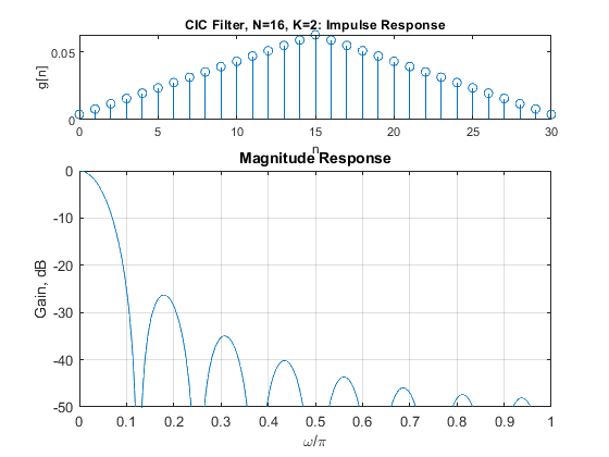
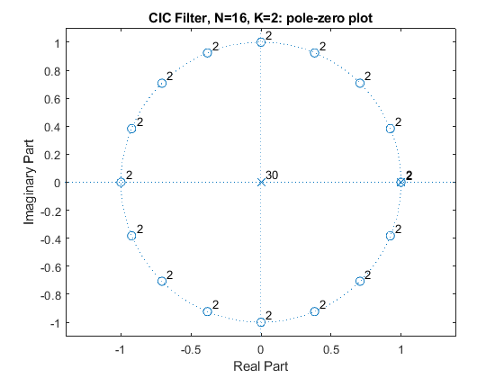
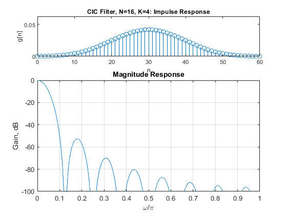
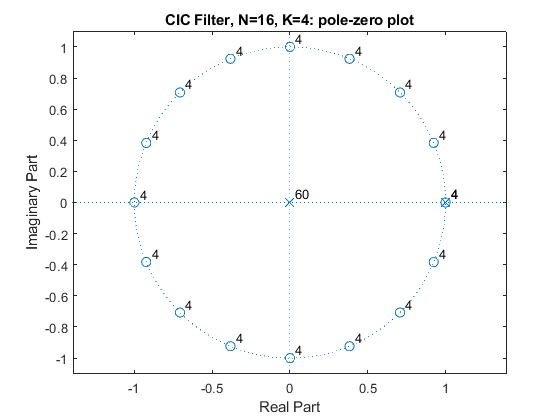
Compute and plot the impulse response, magnitude response, and the pole-zero plot of the K-stage CIC filters G_K(z) for N = 16 and K = 2 and K = 4.

close all, clear all
N=16; K = 2;
g2=conv(rectwin(N)/N,rectwin(N)/N);             % Generating the 2-stage CIC filter impulse response
% Recursive representation of the CIC filter
% G(Z)=(1/N)*(1-z^(-N))/(1-z^-1)=(1/N)*B(z)/A(z)
B = [1,zeros(1,N-1),-1];
B2 = conv(B,B);
A = [1,-1];
A2 = conv(A,A);
[G2,f]=freqz(B2/(N^K),A2,1000,2);
figure(1),
subplot(3,1,1), stem(0:(2*N-2),g2), axis([0,2*N-2,0,1/N]),
xlabel('n'),ylabel('g[n]'),
title('CIC Filter, N=16, K=2: Impulse Response');
subplot(3,1,2:3),
plot(f,20*log10(abs(G2))), xlabel('\omega/\pi'),ylabel('Gain, dB'),
title('Magnitude Response');
axis([0,1,-50,0]), grid,
figure(2),
zplane(B2,A2), title('CIC Filter, N=16, K=2: pole-zero plot');

N=16; K = 4;
g4=conv(g2,g2);                                 % Generating the 4-stage CIC filter impulse response
B4 = conv(B2,B2);
A4 = conv(A2,A2);
[G4,f]=freqz(B4/(N^K),A4,1000,2);
figure(3),
subplot(3,1,1), stem(0:length(g4)-1,g4), axis([0,length(g4)-1,0,1/N]),
xlabel('n'),ylabel('g[n]'),
title('CIC Filter, N=16, K=4: Impulse Response');
subplot(3,1,2:3),
plot(f,20*log10(abs(G4))), xlabel('\omega/\pi'),ylabel('Gain, dB'),
title('Magnitude Response');
axis([0,1,-100,0]), grid,
figure(4),
zplane(B4,A4), title('CIC Filter, N=16, K=4: pole-zero plot');

Exercise 11.3

Modify specifications of Example 11.1 to design a two-stage factor-of-16 decimator consisting of the CIC-based factor-of-8 decimator in the first stage, and the factor-of-two decimator in the second stage.
Design CIC filter G_K(z) and FIR filter T(z).
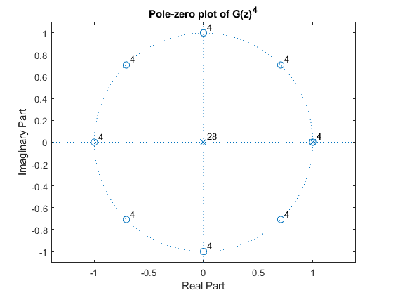
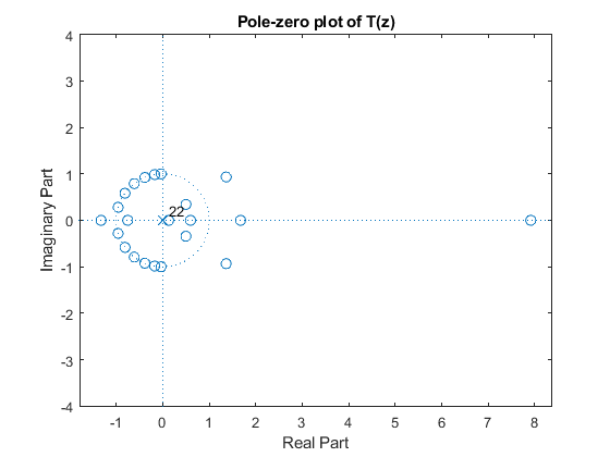
Display the magnitude responses and the pole-zero plots of G_K(z) and T(z).
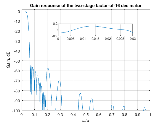
Display the magnitude response of the single-stage equivalent of the resulting overall decimator.

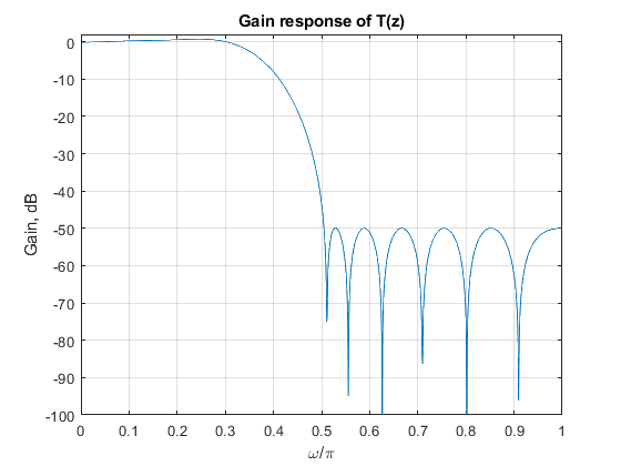
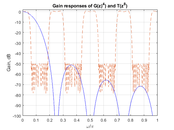
clear all, close all
%
% DESIGN SPECIFICATIONS:
% The overall decimation factor M = 16.
% The overall decimation filter H(z) is specified by:
% Passband edge frequency omega_p = 0.03pi,
% Deviations of the passband magnitude response are bounded to ap = +(-)0.15 dB.
% Stopband edge frequency omega_s = pi/M = 0.0625pi
% Requested minimal stopband attenuation as = 50 dB.
%
% SOLUTION
N = 8; K = 4;                                   % Setting the design parameters for G(z)
B = ([1,zeros(1,N-1),-1]/N); A = [1,-1];        % CIC filter section G(z) = A(z)/B(z)
[G,f] = freqz(B,A,1024,2);                      % Computing the CIC filter frequency response
GK = G.^K;                                      % Computing the frequency response of G_K(z) = G(z)^K
figure(1),
plot(f,20*log10(abs(GK))),
hold on,
xlabel('\omega/\pi'),ylabel('Gain, dB'),
axis([0,1,-100,2]);
% FIR filter T(z)
Nord=22;                                        % Filter order for T(z)
Fo = [0,0.25,0.505,1]; Ao = [0.985,1.09,0,0];   % Setting the specifications for T(z)
t = firpm(Nord,Fo,Ao);                          % Computing the coefficients of T(z)
[T,f]=freqz(t,1,1024,2);                        % Computing the frequency response of T(z)
figure(2),
plot(f,20*log10(abs(T))), grid,
xlabel('\omega/\pi'),ylabel('Gain, dB'),
title('Gain response of T(z)'),
axis([0,1,-100,2]);
figure(1),
tN=upsample(t,N);                               % Computing the coefficients of T(z^N)
[TN,f]=freqz(tN,1,1024,2);                      %  Computing the frequency response of T(z^N)
plot(f,20*log10(abs(TN)),'--',f,20*log10(abs(GK)),'b'), grid,
title('Gain responses of G(z)^4) and T(z^8)'),
axis([0,1,-100,2]);
% Pole-zero plot of G_K(z) = G(z)^K
figure(3),
zplane(conv(conv(B,B),conv(B,B)),conv(conv(A,A),conv(A,A))),
title('Pole-zero plot of G(z)^4');
figure(4),
% Pole-zero plot of T(z)
zplane(t,1),
title('Pole-zero plot of T(z)'),
% Computing the frequency response of the single-stage equivalent of the
% two-stage factor-of-16 decimator:
H = TN.*GK;                                     % Computing the frequency response of (G(z)^K)*T(z^N)
figure(5),
plot(f,20*log10(abs(H))), grid,
xlabel('\omega/\pi'),ylabel('Gain, dB'),
title('Gain response of the two-stage factor-of-16 decimator'),
axis([0,1,-100,2]);
axes('Position',[0.35 0.71 0.45 0.1]);
plot(f(1:54),20*log10(abs(H(1:54)))), axis([0,0.03,-0.2,0.2]),grid;

Exercise 11.4

Consider the polyphase implementation of a CIC filter.
Use equation (11.17a) and MATLAB program of Example 11.2 to compute the coefficients of the FIR transfer function H₁(z) for the following parameters:
(i) N₁ = 4, K = 4;
(ii) N₁ = 8, K = 3.

close all, clear all
% (i) N1 = 4, K = 4
N1 = 4;
g = rectwin(N1); h1 = 1;
K = 4;
for l = 1:K
    h1 = conv(h1,g);
end
disp('Coefficients of the filter impulse tesponse')
disp(['h_1: ' num2str(h1')]);                    % Display the coefficients of the filter impulse response h1

% Polyphase components:
e0 = downsample(h1,4);
e1 = downsample(h1,4,1);
e2 = downsample(h1,4,2);
e3 = downsample(h1,4,3);
disp('Coefficients of the polyphase components')
disp(['e_0: ' num2str(e0')]);
disp(['e_1: ' num2str(e1')]);
disp(['e_2: ' num2str(e2')]);
disp(['e_3: ' num2str(e3')]);                    % Display the coefficients of polyphase components e0, e1, e2, e3

% (ii) N1 = 8, K = 3
N1 = 8;
g = rectwin(N1); h1 = 1;
K = 3;
for l = 1:K
    h1 = conv(h1,g);
end
disp(' ')
disp('Coefficients of the filter impulse tesponse')
disp(['h_1: ' num2str(h1')]);                    % Display the coefficients of the filter impulse response h1

% Polyphase components:
e0 = downsample(h1,N1);
e1 = downsample(h1,N1,1);
e2 = downsample(h1,N1,2);
e3 = downsample(h1,N1,3);
e4 = downsample(h1,N1,4);
e5 = downsample(h1,N1,5);
e6 = downsample(h1,N1,6);
e7 = downsample(h1,N1,7);
% Display the coefficients of polyphase components e0-e7
disp('Coefficients of the polyphase components')
disp(['e_0: ' num2str(e0')]);
disp(['e_1: ' num2str(e1')]);
disp(['e_2= ' num2str(e2')]);
disp(['e_3: ' num2str(e3')]);
disp(['e_4: ' num2str(e4')]);
disp(['e_5: ' num2str(e5')]);
disp(['e_6: ' num2str(e6')]);
disp(['e_7: ' num2str(e7')]);

Coefficients of the filter impulse tesponse
h_1: 1   4  10  20  31  40  44  40  31  20  10   4   1
Coefficients of the polyphase components
e_0: 1  31  31   1
e_1: 4  40  20
e_2: 10  44  10
e_3: 20  40   4
 
Coefficients of the filter impulse tesponse
h_1: 1   3   6  10  15  21  28  36  42  46  48  48  46  42  36  28  21  15  10   6   3   1
Coefficients of the polyphase components
e_0: 1  42  21
e_1: 3  46  15
e_2= 6  48  10
e_3: 10  48   6
e_4: 15  46   3
e_5: 21  42   1
e_6: 28  36
e_7: 36  28

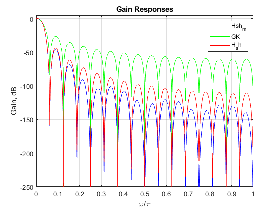
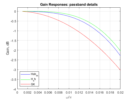
Exercise 11.5

Modify MATLAB program of Example 11.4 to compute and plot the magnitude response for the following decimation filters:
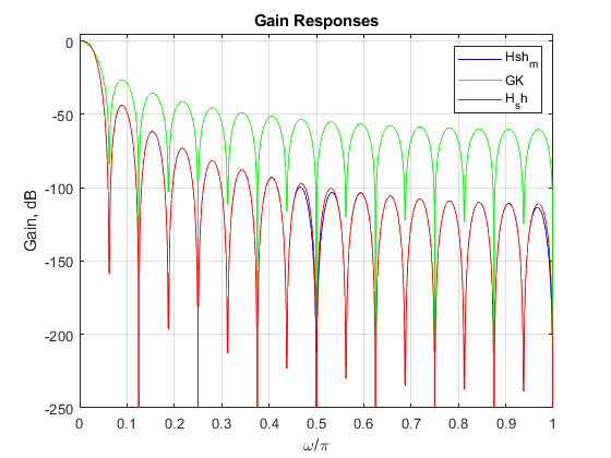
a)   Magnitude response of the modified sharpened CIC filter determined by: N = 32, N₁ = 4, N₂ = 8,
      K = 2, and L = 4.
b)   Magnitude response of the original CIC filter with N = 32, and K = 2.
c)   Magnitude response of the sharpened CIC filter (equations (11.22) and (11.23)) with N = 32,
      and K = 2.

clear all, close all
% Modified sharpened FIR filter
K = 2; N = 32; N1 = 4; N2 = 8; L = 4;           % Setting the design parameters
f = 0:0.001:1;                                  % Setting the frequency axis
omega = pi*f;                                   % Angular frequencies
H1 = (sin(omega*N/2)./sin(omega*N1/2))/N2;      % Amplitude response of the CIC filter H1(z)
H2 = (sin(omega*N1/2)./sin(omega/2))/N1;        % Amplitude response of the CIC filter H2(z)
H_sh_m = abs((3*H1.^(2*K) - 2*H1.^(3*K)).*(H2.^L)); % Magnitude response of the the modified sharpened filter
figure(1),
plot(f,20*log10(H_sh_m),'b'),
axis([0,1,-250,5]), grid,
hold on;
G = (sin(omega*N/2)./sin(omega/2))/N;           % Amplitude response of the original CIC filter
GK = G.^K;                                      % Computing the amplitude response of G(z).^K
plot(f,20*log10(abs(GK)),'g');
H_sh = abs(3*G.^(2*K) - 2*G.^(3*K));            % Magnitude response of the original sharpened CIC filter
plot(f,20*log10(H_sh),'r'), xlabel('\omega/\pi'), ylabel('Gain, dB'),
legend('Hsh_m','GK','H_sh'),
title('Gain Responses');
figure(2),
plot(f(1:21),20*log10(H_sh_m(1:21)),'b'),
hold on;
plot(f(1:21),20*log10(H_sh(1:21)),'g'), xlabel('\omega/\pi'), ylabel('Gain, dB'),
plot(f(1:21),20*log10(abs(GK(1:21))),'r'),
axis([0,0.02,-4,0.2]), grid;
legend('Hsh_m','H_sh','GK','Location','southwest'),
title('Gain Responses: passband details');

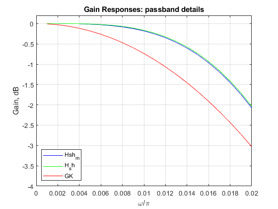
Exercise 11.6

Using the procedure of Exercise 11.5, compute and plot the magnitude response for the following decimation filters:
a)   Magnitude response of the modified sharpened CIC filter determined by: N = 32, N₁ = 4, N₂ = 8,
      K = 2, and L = 5.
b)   Magnitude response of the original CIC filter with N = 32, and K = 2.
c)   Magnitude response of the sharpened CIC filter (equations (11.20) and (11.21)) with N = 32,
      and K = 2.

clear all, close all
% Modified sharpened FIR filter
K = 2; N = 32; N1 = 8; N2 = 4; L = 5;           % Setting the design parameters
f = 0:0.001:1;                                  % Setting the frequency axis
omega = pi*f;                                   % Angular frequencies
H1 = (sin(omega*N/2)./sin(omega*N1/2))/N2;      % Amplitude response of the CIC filter H1(z)
H2 = (sin(omega*N1/2)./sin(omega/2))/N1;        % Amplitude response of the CIC filter H2(z)
H_sh_m = abs((3*H1.^(2*K)-2*H1.^(3*K)).*(H2.^L)); % Magnitude response of the modified sharpened filter
figure(1),
plot(f,20*log10(H_sh_m),'b'),
axis([0,1,-250,5]), grid,
hold on;
G = (sin(omega*N/2)./sin(omega/2))/N;           % Amplitude response of the original CIC filter
GK = G.^K;                                      % Computing the amplitude response of G(z).^K
plot(f,20*log10(abs(GK)),'g')
H_sh = abs(3*G.^(2*K) - 2*G.^(3*K));            % Magnitude response of the original sharpened CIC filter
plot(f,20*log10(H_sh),'r'), xlabel('\omega/\pi'), ylabel('Gain, dB'),
legend('Hsh_m','GK','H_sh'),
title('Gain Responses');
figure(2),
plot(f(1:21),20*log10(H_sh_m(1:21)),'b'),
hold on;
plot(f(1:21),20*log10(H_sh(1:21)),'g'), xlabel('\omega/\pi'), ylabel('Gain, dB'),
plot(f(1:21),20*log10(abs(GK(1:21))),'r'),
axis([0,0.02,-4,0.2]), grid,
legend('Hsh_m','H_sh','GK','Location','southwest'),
title('Gain Responses: passband details');

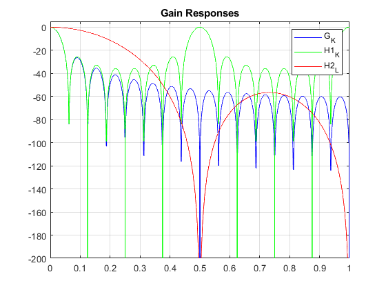
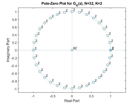
Exercise 11.7

Display the magnitude response and pole-zero plot of the CIC filter G_K(z) determined by N = 32 and K = 2.
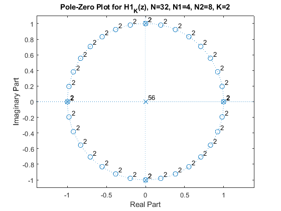
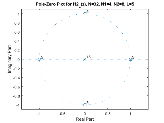
Compose the CIC subfilters [H₁(z^N1)]^K and [H₂(z)]^L of the modified sharpened filter as given in equations (11.27) and (11.28).
Compute and plot the magnitude responses and pole-zero plots of [H₁(z^N1)]^K and [H₂(z)]^L for the parameters N = 32, N₁ = 4, N₂ = 8, K = 2, and L = 5.

clear all, close all
% Modified sharpened FIR filters
K = 2; N = 32; N1 = 4; N2 = 8; L = 5;           % Setting the design parameters
f = 0:0.001:1;                                  % Setting the frequency axis
omega = pi*f;                                   % Angular frequencies
G = (sin(omega*N/2)./sin(omega/2))/N;           % Amplitude response of the original CIC filter
G_K = G.^K;                                     % Computing the amplitude response of G(z).^K
H1 = (sin(omega*N/2)./sin(omega*N1/2))/N2;      % Amplitudee response of the CIC filter H1(z)
H1_K = H1.^K;
H2 = (sin(omega*N1/2)./sin(omega/2))/N1;        % Amplitude response of the CIC filter H2(z)
H2_L = H2.^L;
figure(1),
plot(f,20*log10(abs(G_K)),'b'),
hold on,
plot(f,20*log10(abs(H1_K)),'g')
axis([0,1,-200,5]), grid,
plot(f,20*log10(abs(H2_L)),'r'),
legend('G_K','H1_K','H2_L'),
title('Gain Responses');
% Computing the pole-zero plot for G_K(z), H1_K, and H2_L
% Recursive representation of the CIC filter
% G_K(Z)=(1/N)*(1-z^(-N))/(1-z^-1)=(1/N)*B(z)/A(z), K=2
B = [1,zeros(1,N-1),-1];
B2 = conv(B,B);
A = [1,-1];
A2 = conv(A,A);
figure(2),
zplane(B2,A2),
title('Pole-Zero Plot for G_K(z), N=32, K=2');
% Recursive representation of the filter H1_K, N=32, N1=4, N2=8, K=2
% H1_K(Z)=(1/N2)*(1-z^(-N))/(1-z^-N1)=(1/N2)*B(z)/A(z)
B = [1,zeros(1,N-1),-1];
B2 = conv(B,B);
A = [1,zeros(1,N1-1),-1];
A2 = conv(A,A);
figure(3),
zplane(B2,A2),
title('Pole-Zero Plot for H1_K(z), N=32, N1=4, N2=8, K=2');
% Recursive representation of the filter H2_L, N=32, N1=4, N2=8, K=2
% H2_L(Z)=(1/N1)*(1-z^(-N1))/(1-z^-1)=(1/N1)*B(z)/A(z)
B = [1,zeros(1,N1-1),-1];
BL = conv(B,B); BL=conv(BL,BL); BL=conv(BL,B);
A = [1,-1];
AL = conv(A,A); AL=conv(AL,AL); AL=conv(AL,A);
figure(4),
zplane(BL,AL),
title('Pole-Zero Plot for H2_L(z), N=32, N1=4, N2=8, L=5');