Multirate Filtering for Digital Signal Processing: MATLAB® Applications, Chapter 10: Frequency-Response Masking Techniques - Exercises
Contents
Exercise 10.1
Use the MATLAB function ifir to design
a lowpass FIR filter to satisfy the specifications of Example 10.1.
Compute and plot the magnitude response of the overall lowpass filter and
compare the results with that of Example 10.1.
Used function: ifir (DSP System Toolbox), freqz (Signal Processing Toolbox)
close all; clear all;
%
% Specifications of Example 10.1
% A lowpass FIR filter is designed for Fp = 100 Hz, Fs = 150 Hz, and the sampling frequency of F0 = 2000 Hz.
% The passband and stopband ripples are delta_p = 0.01, and delta_s = 0.01 (a_s = 40 dB).
%
Fp=100; Fs=150; F0=2000;
delta_p=0.01; delta_s=0.01;
% SOLUTION
[g,h] = ifir(4,'low',[Fp/(F0/2),Fs/(F0/2)],[delta_p,delta_s]);
hIFIR = conv(g,h);
[HIFIR,f] = freqz(hIFIR,1,1000,F0);
figure(1),plot(f,20*log10(abs(HIFIR))),
xlabel('Frequency [Hz]'),ylabel('Gain [dB]');
axis([0,F0/2,-60,5]),grid on;
g(1)=axes('Position',[0.40 0.70 0.40 0.1]);
plot(f(1:100),(abs(HIFIR(1:100)))),axis([0,100,0.99,1.01]);
% Figure 1 displays the gain response of the overall filter, which
% evidently meets the speciffications.
% The plots of Figure 1 are simmilar to those of Figure 10.4 which presents
% the solution of Example 10.1 (from the book).
Exercise 10.2
Design a narrowband filter for the
specifications of Example 10.1.
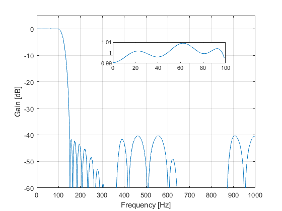
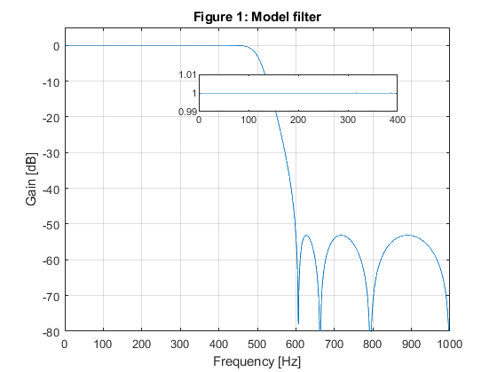
The model filter G(z) is an IIR halfband filter,
and masking filter F(z) is a linear-phase FIR filter.
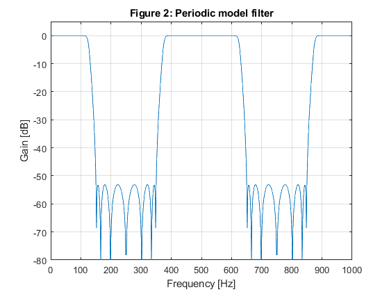
Compute and plot the magnitude responses for G(z), G(zM),
F(z), and for the overall filter H(z).
Compute the total number of multiplication constants and compare with the
solution of Example 10.1.
Used function: halfbandiir, freqz (Signal Processing Toolbox), fminimax, options (Optimization Toolbox), halfbandiir (Appendix)
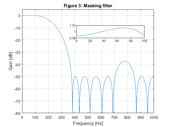
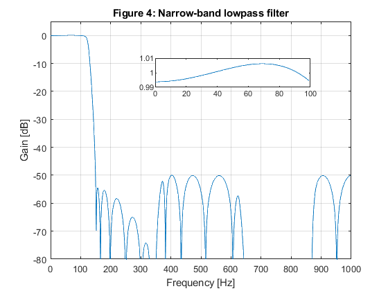
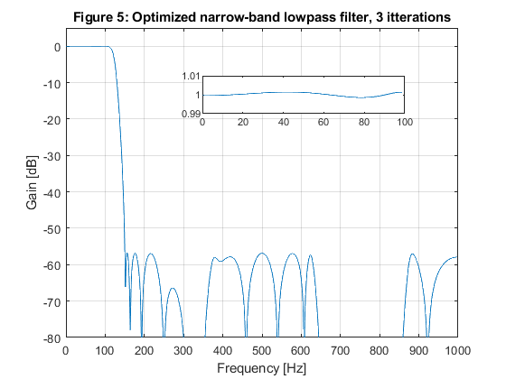
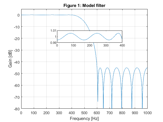
close all; clear all;
%
% Specifications of Example 10.1
% A lowpass FIR filter is designed for Fp = 100 Hz, Fs = 150 Hz, and the sampling frequency of F0 = 2000 Hz.
% The passband and stopband ripples are delta_p = 0.01, and delta_s = 0.01 (a_s = 40 dB).
%
Fp=100; Fs=150; F0=2000;
delta_p=0.01; delta_s=0.01;
% SOLUTION
Ng = 7;                                     % The order of the IIR model filter
[b,a,z,p,k] = halfbandiir(Ng,400/(F0/2));   % Model filter
[G,f] = freqz(b,a,1000,F0);
figure(1),plot(f,20*log10(abs(G))),
xlabel('Frequency [Hz]'),ylabel('Gain [dB]'),
axis([0,F0/2,-80,5]),grid on,
title('Figure 1: Model filter');
g(1)=axes('Position',[0.40 0.70 0.40 0.1]);
plot(f(1:400),(abs(G(1:400)))), axis([0,400,0.99,1.01]);
M = 4;

% Generating the periodic model filter
bm = zeros(size(1:M*length(b)));
bm(1:M:length(bm)) = b;
am = zeros(size(1:M*length(a)));
am(1:M:length(am)) = a;
[Gm,f] = freqz(bm,am,1000,F0);
figure(2),plot(f,20*log10(abs(Gm))),
xlabel('Frequency [Hz]'),ylabel('Gain [dB]'),
axis([0,F0/2,-80,5]),grid on,
title('Figure 2: Periodic model filter');

% Design of the masking filter
f0=[0,100/1000,375/1000,650/1000,850/1000,1]; m0=[1,1,0,0,0,0];
Nf = 19; % Length of FIR linear-phase masking filtr
ff = firpm(Nf-1,f0,m0,[0.5,1,1]);
[F,f]=freqz(ff,1,1000,F0);
figure(3),plot(f,20*log10(abs(F))),
xlabel('Frequency [Hz]'),ylabel('Gain [dB]'),
axis([0,F0/2,-80,5]),grid on,
title('Figure 3: Masking filter');
g(1)=axes('Position',[0.45 0.70 0.40 0.1]);
plot(f(1:100),(abs(F(1:100)))), axis([0,100,0.99,1.01]);

% Narrow-band lowpass filter characteristic
H=F.*Gm;
figure(4),plot(f,20*log10(abs(H))),
xlabel('Frequency [Hz]'),ylabel('Gain [dB]'),
axis([0,1000,-80,5]),grid on,
title('Figure 4: Narrow-band lowpass filter');
g(1)=axes('Position',[0.40 0.70 0.40 0.1]);
plot(f(1:100),(abs(H(1:100)))), axis([0,100,0.99,1.01]);

% Computing the number of multiplication constants N_MULT:
N_MULT = (Ng-1)/2 + (Nf-1)/2 +1
% The total number of multiplication constants is N_MULT = 13, whereas
% the number of multiplication constants in the solution of Example 10.1
% is 16.
%
% OPTIMIZATION
x0 = [b,a(3),a(5),a(7),ff(1:10)];
options = optimset('MinAbsMax',length(1:1000),'TolFun',1e-4,'TolCon',1e-4,'MaxIter',20);
[x,Err,maxfval,exitflag,output] = fminimax(@ErrLP,x0,[],[],[],[],[],[],[],options);
b = x(1:8); a = [1,0,x(9),0,x(10),0,x(11),0]; ff = [x(12:21),fliplr(x(12:20))];
bm = zeros(size(1:M*length(b)));
bm(1:M:length(bm)) = b;
am = zeros(size(1:M*length(a)));
am(1:M:length(am)) = a;
[Gm,f] = freqz(bm,am,1000,F0);
[F,f]=freqz(ff,1,1000,F0);
H=F.*Gm;
figure(5),plot(f,20*log10(abs(H))),
xlabel('Frequency [Hz]'),ylabel('Gain [dB]'),
axis([0,1000,-80,5]),grid on,
title('Figure 5: Optimized narrow-band lowpass filter, 3 itterations');
g(1)=axes('Position',[0.40 0.70 0.40 0.1]);
plot(f(1:100),(abs(H(1:100)))), axis([0,100,0.99,1.01]);
N_MULT =

    13


Local minimum possible. Constraints satisfied.

fminimax stopped because the predicted change in the objective function
is less than the value of the function tolerance and constraints
are satisfied to within the value of the constraint tolerance.
Exercise 10.3
Using the frequency-response masking approach design a highpass FIR filter to
satisfy the following specifications:
Fp = 900 Hz, Fs = 850 Hz, and the sampling frequency of F0 = 2000 Hz.
The passband and stopband ripples are δp = 0.01, and δs = 0.01 (as = 40 dB).
Compute and plot the magnitude responses for the following filters:
model filter, periodic model filter, masking filter, and for the
resulting highpass filter.
Used function: firhalfband (DSP System Toolbox), freqz (Signal Processing Toolbox), fminimax, options (Optimization Toolbox)
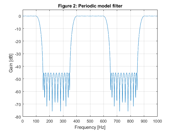
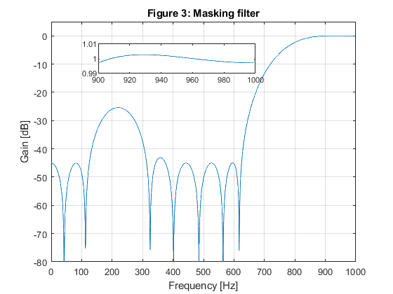
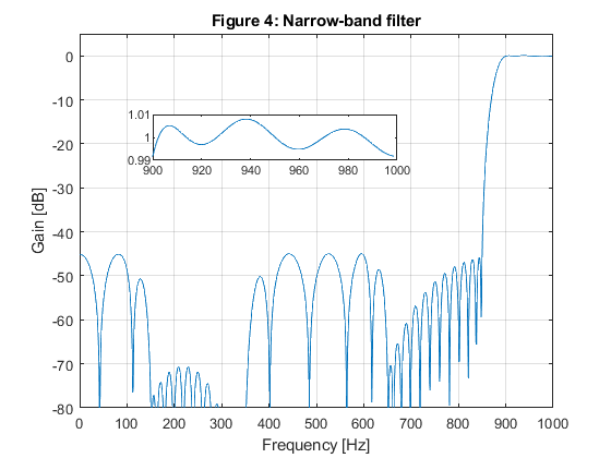
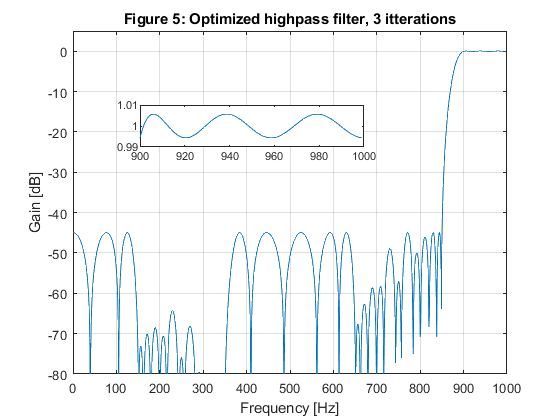
close all; clear all;
% SOLUTION
gg = firhalfband(22,400/1000);               % Model filter
[G,f]=freqz(gg,1,1000,2000);
figure(1),plot(f,20*log10(abs(G))),
xlabel('Frequency [Hz]'),ylabel('Gain [dB]'),
axis([0,1000,-80,5]),grid on,
title('Figure 1: Model filter');
g(1)=axes('Position',[0.35 0.65 0.40 0.1]);
plot(f(1:400),(abs(G(1:400)))), axis([0,400,0.99,1.01]);

% Generation of the periodic model filter
gm = zeros(size(1:4*length(gg)));
gm(1:4:length(gm)) = gg;
[Gm,f]=freqz(gm,1,1000,2000);
figure(2),plot(f,20*log10(abs(Gm))),
xlabel('Frequency [Hz]'),ylabel('Gain [dB]'),
axis([0,1000,-80,5]),grid on,
title('Figure 2: Periodic model filter');

% Design of the highpass masking filter
f0=[0,125/1000,375/1000,625/1000,900/1000,1]; m0=[0,0,0,0,1,1];
ff = firpm(18,f0,m0,[0.5,0.5,1]);
[F,f] = freqz(ff,1,1000,2000);
figure(3),plot(f,20*log10(abs(F))),
xlabel('Frequency [Hz]'),ylabel('Gain [dB]'),
axis([0,1000,-80,5]),grid on,
title('Figure 3: Masking filter');
g(1)=axes('Position',[0.25 0.75 0.40 0.1]);
plot(f(900:1000),(abs(F(900:1000)))), axis([900,1000,0.99,1.01]);

% Highpass filter characteristic
H = F.*Gm;
figure(4),plot(f,20*log10(abs(H))),
xlabel('Frequency [Hz]'),ylabel('Gain [dB]'),
axis([0,1000,-80,5]),grid on,
title('Figure 4: Narrow-band filter');
g(1)=axes('Position',[0.25 0.65 0.40 0.1]);
plot(f(900:1000),(abs(H(900:1000)))), axis([900,1000,0.99,1.01]);

% OPTIMIZATION
x0 = [gg(1:2:11),ff(1:10)];
options = optimset('MinAbsMax',length(1:1000),'TolFun',1e-6,'TolCon',1e-6,'MaxIter',10);
[x,Err,maxfval,exitflag,output] = fminimax(@ErrHP,x0,[],[],[],[],[],[],[],options);

% Frequency response of the optimized highpass filter
gg = zeros(size(1:11));
gg(1:2:11) = x(1:6);
gg = [gg,0.5,fliplr(gg)];
ff = [x(7:16),fliplr(x(7:15))];
gm = zeros(size(1:4*length(gg)));
gm(1:4:length(gm)) = gg;
[Gm,f]= freqz(gm,1,1000,2000);
[F,f] = freqz(ff,1,1000,2000);
H = Gm.*F;
figure(5),plot(f,20*log10(abs(H)))
xlabel('Frequency [Hz]'),ylabel('Gain [dB]'),
axis([0,1000,-80,5]),grid on,
title('Figure 5: Optimized highpass filter, 3 itterations');
g(1)=axes('Position',[0.25 0.65 0.40 0.1]);
plot(f(900:1000),(abs(H(900:1000)))), axis([900,1000,0.99,1.01])
Local minimum possible. Constraints satisfied.

fminimax stopped because the size of the current search direction is less than
twice the value of the step size tolerance and constraints are
satisfied to within the value of the constraint tolerance.
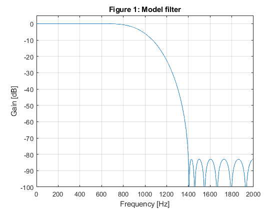
Exercise 10.4
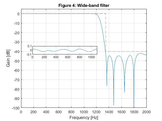
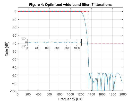
Design a wideband linear-phase lowpass filter
specified with the passband edge frequency Fp = 1100 Hz,
the stopband edge frequency Fs = 1350 Hz
and the sampling frequency F0 = 4000 Hz.
The maximal ripple in the passband is ap = ±0.1 dB,
and minimal stopband attenuation amounts to as = 40 dB.
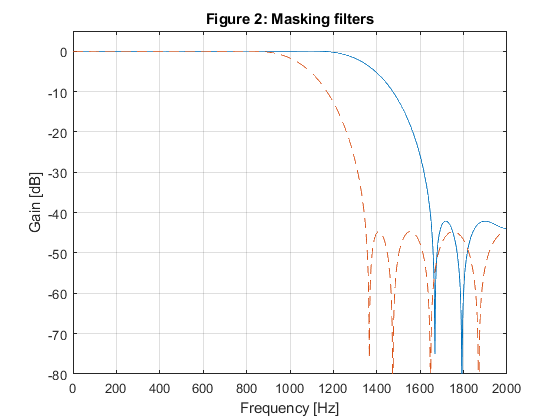
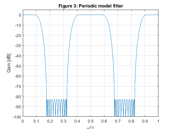
Compute and plot the magnitude responses for the following filters:
Model filter, periodic model filter, masking filters,
and for the resulting lowpass filter.
Used function: firhalfband (DSP System Toolbox), freqz (Signal Processing Toolbox), fminimax, options (Optimization Toolbox)
close all; clear all;
% SOLUTION
% Design od the model filter
omegap = 2*pi*1100/4000;
omegas = 2*pi*1350/4000;
M = 4;                                      % We chose
omegaGs = omegas*M - 2*pi;                  % Model filter stopband angular edge frequency
fGs = omegaGs/pi;                           % Model filter stopband edge frequency
omegaGp = omegap*M - 2*pi;                  % Model filter passband angular edge frequency
fGp = omegaGp/pi;                           % Model filter passpband edge frequency
% Selecting the suitable passband edge frequency for the halfband model filter:
if 1-fGs>=fGp,
    fGp = 1-fGs;
end;
%fGp = 1-fGs;                               % Model filter passband edge frequency
g = firhalfband(22,fGp);                    % Model filter design
[G,fr] = freqz(g,1,1000,4000);
figure(1),plot(fr,20*log10(abs(G))),
xlabel('Frequency [Hz]'),ylabel('Gain [dB]'),
axis([0,2000,-100,5]),grid on,
title('Figure 1: Model filter');

% Design of the masking filters F0(z) and F1(z)
ap = 0.08; as = 40;
delta_p = (10^(ap/20)-1)/(10^(ap/20)+1);    % Passband ripple
delta_s = 10^(-as/20);                      % Stopband ripple
fpF0 = (2+fGp)/M; fsF0 = (4-fGs)/M;         % Boundary frequencies for filter F0(z)
freq = [0,fpF0,fsF0,1]; m0 = [1,1,0,0]; w = [delta_s/delta_p,1]; % Seting design parameters for masking filter F0(z)
f0 = firpm(18,freq,m0,w);                   % Designing the masking filter f0
fpF1 = (2-fGp)/M; fsF1 = (2+fGs)/M;         % Boundary frequencies for filter F1(z)
freq = [0,fpF1,fsF1,1]; m1=[1,1,0,0];       % Seting design parameters for masking filter  F1(z
f1 = firpm(20,freq,m1,w);                   % Designing the masking filter f1
[F0,fr] = freqz(f0,1,1000,4000);
[F1,fr] = freqz(f1,1,1000,4000);
figure(2),plot(fr,20*log10(abs(F0)),fr,20*log10(abs(F1)),'--');grid
xlabel('Frequency [Hz]'),ylabel('Gain [dB]'),
axis([0,2000,-80,5]),grid on,
xlabel('Frequency [Hz]'),ylabel('Gain [dB]'),
title('Figure 2: Masking filters');
f0=[0,f0,0];                                % Equalization of the masking filters' delays

% Generation of the periodic model filter
gm = zeros(size(1:4*length(g)));
gm(1:4:length(gm)) = g;                   % Periodic model filter
[Gm,fr] = freqz(gm,1,1024,2);
figure(3),plot(fr,20*log10(abs(Gm)));
xlabel('\omega/\pi'),ylabel('Gain [dB]'),
axis([0,1,-100,5]),grid on,
title('Figure 3: Periodic model filter');

% Implementation of the wideband filter according to Figure 10.8
d = zeros(size(gm)); d(45) = 1;             % Delay branch
gmc = d - gm;                               % Complementary periodic model filter
[Gmc,fr]=freqz(gmc,1,1000,4000);
h = conv(gm,f0) + conv(gmc,f1);             % Impulse response of the overall filter
[H,Fr]=freqz(h,1,1000,4000);
figure(4),plot(Fr,20*log10(abs(H))),
xlabel('Frequency [Hz]'),ylabel('Gain [dB]')
hold on
plot([0,1350,1350,2000],[0,0,-40,-40],'r--'),
axis([0,2000,-100,5]), grid on,
title('Figure 4: Wide-band filter');
g(1)=axes('Position',[0.20 0.55 0.40 0.07]);
plot(Fr(1:550),20*log10(abs(H(1:550)))),axis([0,1100,-0.1,0.1]);

% OPTIMIZATION
x0 = [g(1:2:11),f0(2:11),f1(1:11)];
options = optimset('MinAbsMax',length(1:1000),'TolFun',1e-5,'TolCon',1e-5,'MaxIter',20);
[x,Err,maxfval,exitflag,output] = fminimax(@ErrWB,x0,[],[],[],[],[],[],[],options);

% Frequency response of the optimized wide-band filter
gg = zeros(size(1:11));
gg(1:2:11) = x(1:6);
gg = [gg,0.5,fliplr(gg)];
ff0 = [0,x(7:16),fliplr(x(7:15)),0];
ff1 = [x(17:27),fliplr(x(17:26))];
gm = zeros(size(1:4*length(gg)));
gm(1:4:length(gm)) = gg;
d = zeros(size(gm)); d(45) = 1;
gmc = d - gm;
h = conv(gm,ff0) + conv(gmc,ff1);
[H,Fr]=freqz(h,1,1000,4000);
figure(5),plot(Fr,20*log10(abs(H))),
xlabel('Frequency [Hz]'),ylabel('Gain [dB]')
hold on
plot([0,1350,1350,2000],[0,0,-40,-40],'r--'),
axis([0,2000,-100,5]), grid on,
title('Figure 4: Optimized wide-band filter, 7 itterations');
g(1)=axes('Position',[0.20 0.55 0.40 0.07]);
plot(Fr(1:550),20*log10(abs(H(1:550)))),axis([0,1100,-0.01,0.01]);
%
function Err = ErrWB(x)
gg = zeros(size(1:11));
gg(1:2:11) = x(1:6);
gg = [gg,0.5,fliplr(gg)];
ff0 = [0,x(7:16),fliplr(x(7:15)),0];
ff1 = [x(17:27),fliplr(x(17:26))];
gm = zeros(size(1:4*length(gg)));
gm(1:4:length(gm)) = gg;
d = zeros(size(gm)); d(45) = 1;
gmc = d - gm;
h = conv(gm,ff0) + conv(gmc,ff1);
[H,Fr]=freqz(h,1,1000,4000);
H = abs(H);
Err = [abs(1-H(1:560)'),zeros(size(561:674)),H(675:1000)'];
end
%
function Err = ErrHP(x)
gg = zeros(size(1:11));
gg(1:2:11) = x(1:6);
gg = [gg,0.5,fliplr(gg)];
ff = [x(7:16),fliplr(x(7:15))];
gm = zeros(size(1:4*length(gg)));
gm(1:4:length(gm)) = gg;
[Gm,f]= freqz(gm,1,1000);
[F,f] = freqz(ff,1,1000);
H = Gm.*F;
H = abs(H);
Err = [H(1:850)',zeros(size(851:900)),abs(1-H(901:1000)')];
end
%
function Err = ErrLP(x)
b = x(1:8); a = [1,0,x(9),0,x(10),0,x(11),0]; ff = [x(12:21),fliplr(x(12:20))];
M = 4;
bm = zeros(size(1:M*length(b)));
bm(1:M:length(bm)) = b;
am = zeros(size(1:M*length(a)));
am(1:M:length(am)) = a;
[Gm,f] = freqz(bm,am,1000);
[F,f]=freqz(ff,1,1000);
H=F.*Gm;
H = abs(H);
Err = [abs(1-H(1:100)'),zeros(size(101:150)),H(151:1000)'];
end
Local minimum possible. Constraints satisfied.

fminimax stopped because the predicted change in the objective function
is less than the value of the function tolerance and constraints
are satisfied to within the value of the constraint tolerance.